Thinking in Python Runtime: How an Enterprise AI Application Occupies a Multi-Processor, Multi-Core System

Publication Date: October 05, 2026 Last Updated: October 05, 2026
Hardware and Runtime Fundamentals
Before examining how a Python AI application occupies a multi-processor, multi-core system, it is useful to establish a few foundational concepts. Terms such as CPU socket, physical core, logical CPU, NUMA node, cache, memory bandwidth, PCIe, and GPU are often used interchangeably in architectural discussions, but they describe different layers of the system.
This section establishes the terminology used throughout the article. The goal is not to provide a comprehensive treatment of computer architecture, but to build the minimum mental model required to understand the execution diagrams that follow.
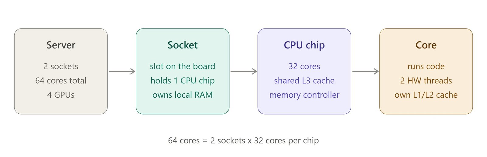
A CPU socket is the physical slot on a server's motherboard into which one processor chip is installed. "Two CPU sockets" means the server has two separate processor chips, each plugged into its own slot. (It has nothing to do with network sockets in programming, which is an unrelated use of the same word.)
If you say "64 cores across two sockets", it means each chip contributes 32 cores. The schematic below zooms in from the server down to a single core.
Next is the physical view of those two sockets on the motherboard. Each socket has its own memory and its own PCIe lanes to the GPUs, and the two are joined by a link between the chips.
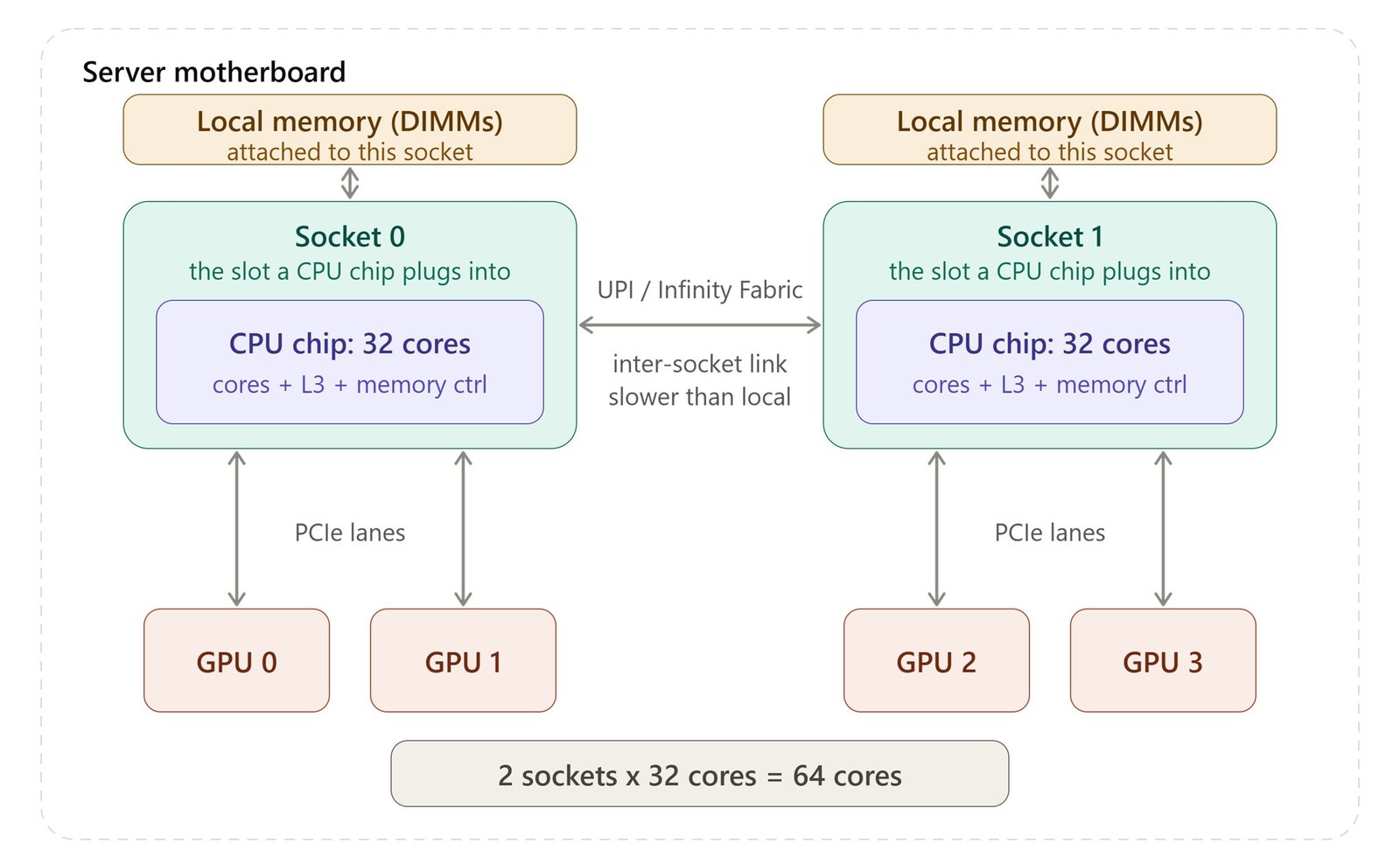
The two sockets are not one pool of 64 equal cores. Each chip reaches its own memory and GPUs quickly, but anything on the other socket has to cross the inter-socket link, which is slower. A service tuned for ten requests per minute on a laptop therefore will not scale just because it lands on a bigger machine. How the workload is placed across the sockets decides the result, and that is the point Figure 1 (Section: Start with the Hardware: Topology Determines Placement) of this article builds on.
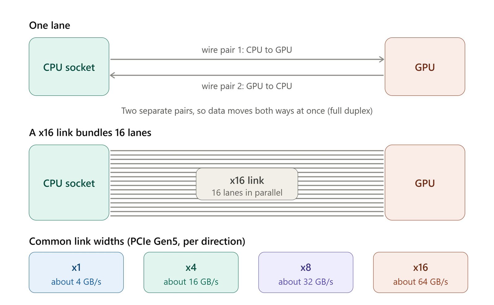
PCIe (PCI Express) is the high-speed connection between a CPU and the devices attached to it, such as GPUs, network cards and NVMe SSDs. A lane is its basic building block. One lane is two pairs of wires, one for sending and one for receiving, so data flows in both directions at the same time. A device connects through a bundle of lanes, written x1, x4, x8 or x16, and more lanes means more bandwidth.
Lanes are a fixed budget per socket and cannot be borrowed from the other socket. Each socket has its own memory and its own PCIe lanes to the GPUs, and the two are joined by a link between the chips. This means GPU 0 and GPU 1 talk to the CPU directly through socket 0's lanes, and GPU 2 and GPU 3 do the same through socket 1's lanes. If a process running on socket 1 needs data in a GPU attached to socket 0, the traffic also has to cross the inter-socket link. That adds latency and competes for the link's bandwidth. This is why pinning each worker to the socket that owns its GPU matters.
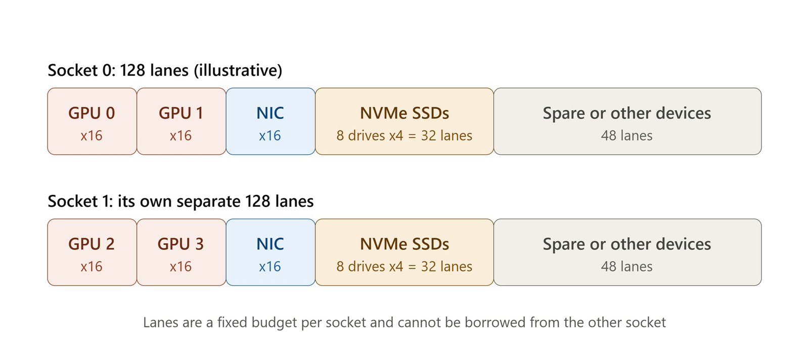
The lane counts in the above diagram are illustrative. Real server CPUs offer anywhere from several dozen to over a hundred lanes per socket, depending on the model.
A CPU core is an independent processing unit inside a CPU chip. It can fetch instructions, decode them, execute them and store the results, all on its own. A chip with 32 cores is like a workshop with 32 separate workers, each with a private workbench (registers and small caches), who share a common storeroom (L3 cache and memory). Each core can run a different program, or a different thread of the same program, at the same time as the others.
The diagram below opens up one core and shows how it relates to the rest of the chip.
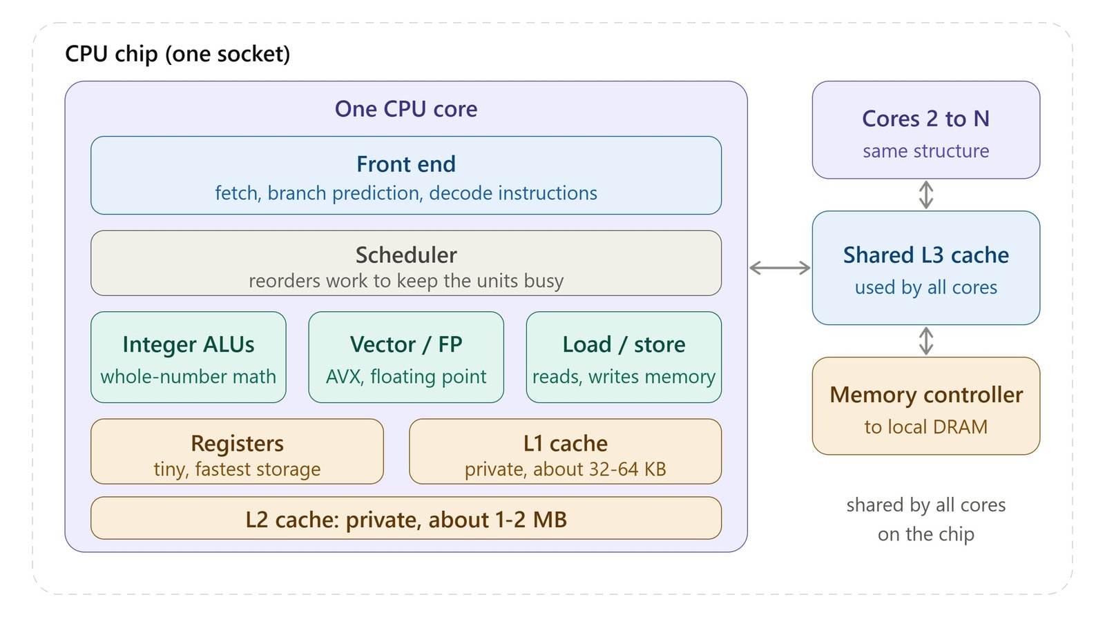
The terms nest as follows: a server contains sockets, each socket holds one CPU chip, each chip holds cores, and with SMT each core presents two logical CPUs. With SMT enabled, the operating system would list 128 logical CPUs, and tools such as lscpu report both numbers. SMT typically improves throughput by a modest margin for mixed workloads, but it does not make a core twice as fast, so capacity planning should count physical cores.
For the Python runtime, the CPU core is where execution happens. Each Python thread is an OS thread that the scheduler places on one logical CPU at a time, and the GIL limits how many of those threads can run bytecode at once. A multi-process design uses several cores in parallel, one interpreter per core, which is why pinning workers to specific cores works so well.
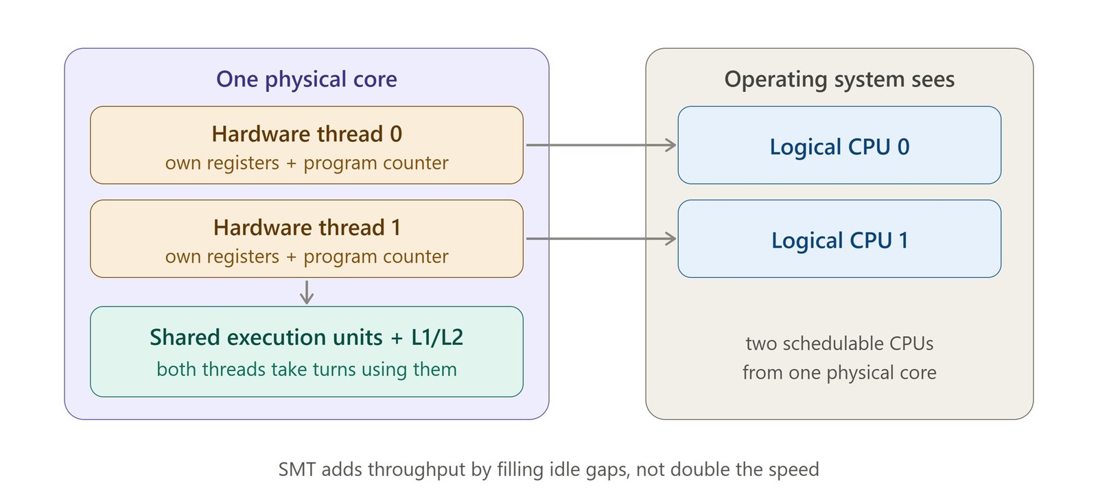
SMT stands for Simultaneous Multithreading. It is a CPU feature that lets one physical core work on two threads at the same time. Intel markets its version as Hyper-Threading, while AMD simply calls it SMT. Each hardware thread keeps its own registers and program counter, but the two share the core's execution units and caches. The operating system then sees one physical core as two logical CPUs, which is what the sentence means by "each core presents two logical CPUs."
The motivation is that a single thread rarely keeps a core fully busy. It stalls while waiting for data from memory, after a mispredicted branch, or on instructions that depend on earlier results. SMT lets a second thread use the execution slots that would otherwise sit idle.
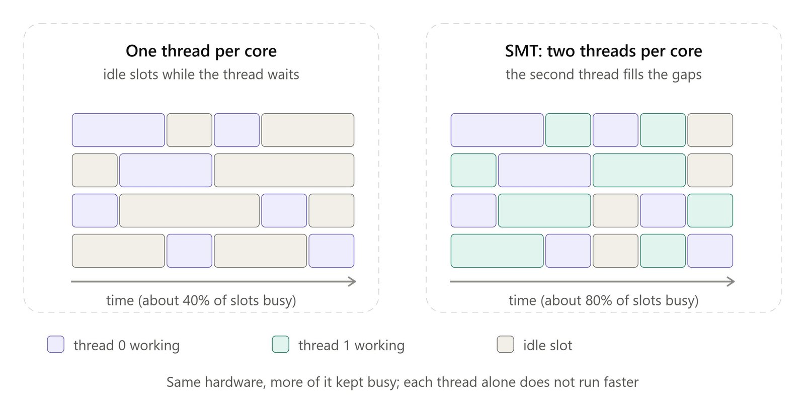
The busy percentages in the diagram are illustrative. In practice SMT raises a core's total throughput by a modest margin that depends heavily on the workload, often somewhere around 10 to 30 percent. It never doubles the speed, because the two threads share the same execution units.
For the Python and AI workloads in this article, this has three practical consequences:
- Count physical cores when sizing. A server with 64 physical cores shows 128 logical CPUs, but the extra 64 are not equivalent to additional cores.
- Heavy numerical work may gain little. Native libraries such as BLAS and PyTorch's CPU kernels already keep a core's vector units busy, so a second thread has few gaps to fill and mostly competes for the same resources.
- Latency-sensitive services often pin workers to physical cores. Placing one worker per physical core avoids two busy threads sharing one core's resources, and some operators turn SMT off for that reason.
NUMA stands for Non-Uniform Memory Access. A NUMA node is a group of CPU cores together with the memory that is directly attached to them. In most two-socket servers each socket forms one NUMA node, although some processors can split a single socket into several nodes. Cores reach memory in their own node quickly. Reaching memory that belongs to another node takes longer because the request has to travel across the link between the chips.
The diagram below contrasts this with the older uniform design, where every core reached one shared pool at the same speed.
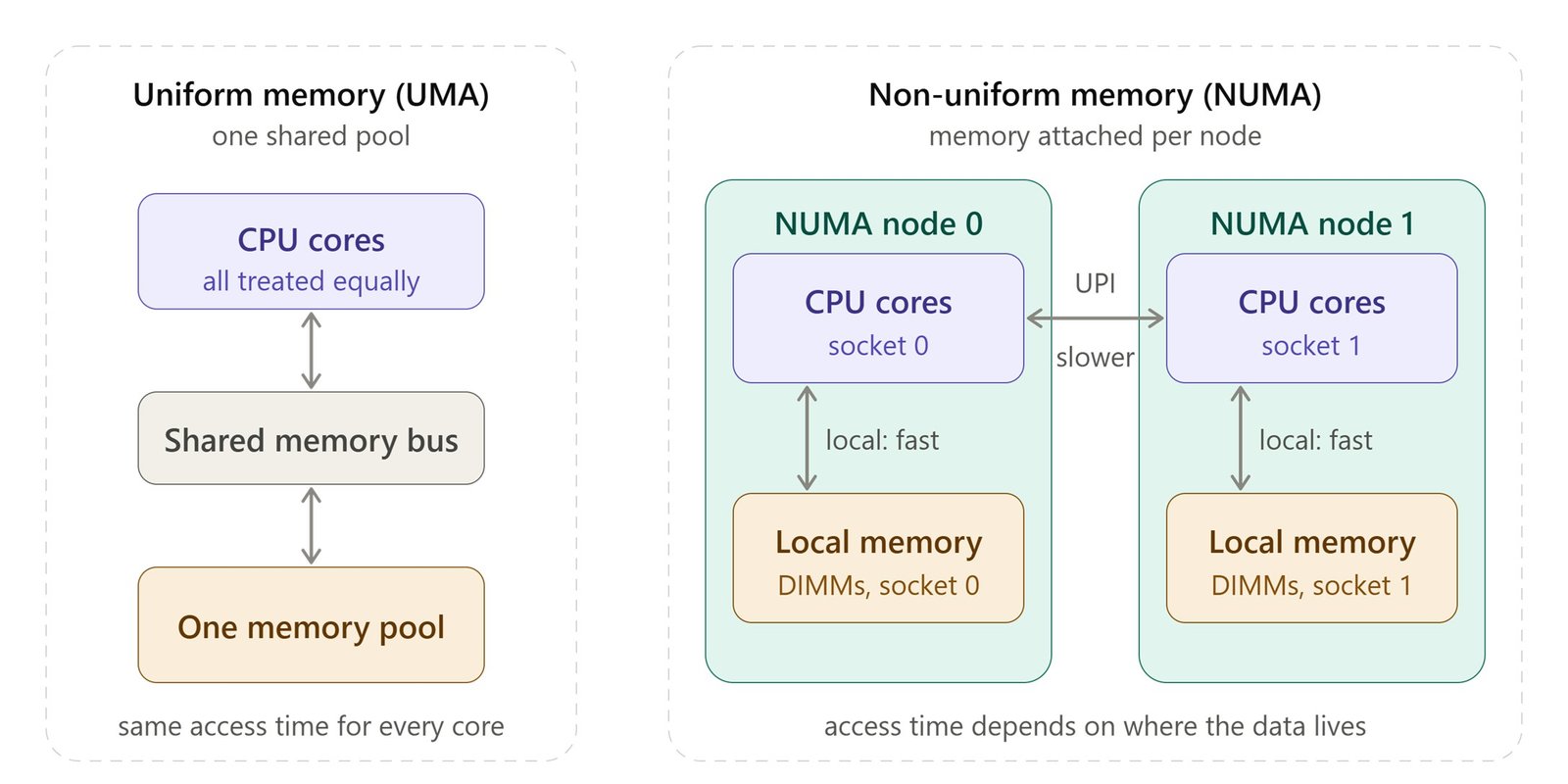
The diagram below shows the same thread reading two pieces of data. Data A sits in its own node's memory. Data B sits in the other node's memory.
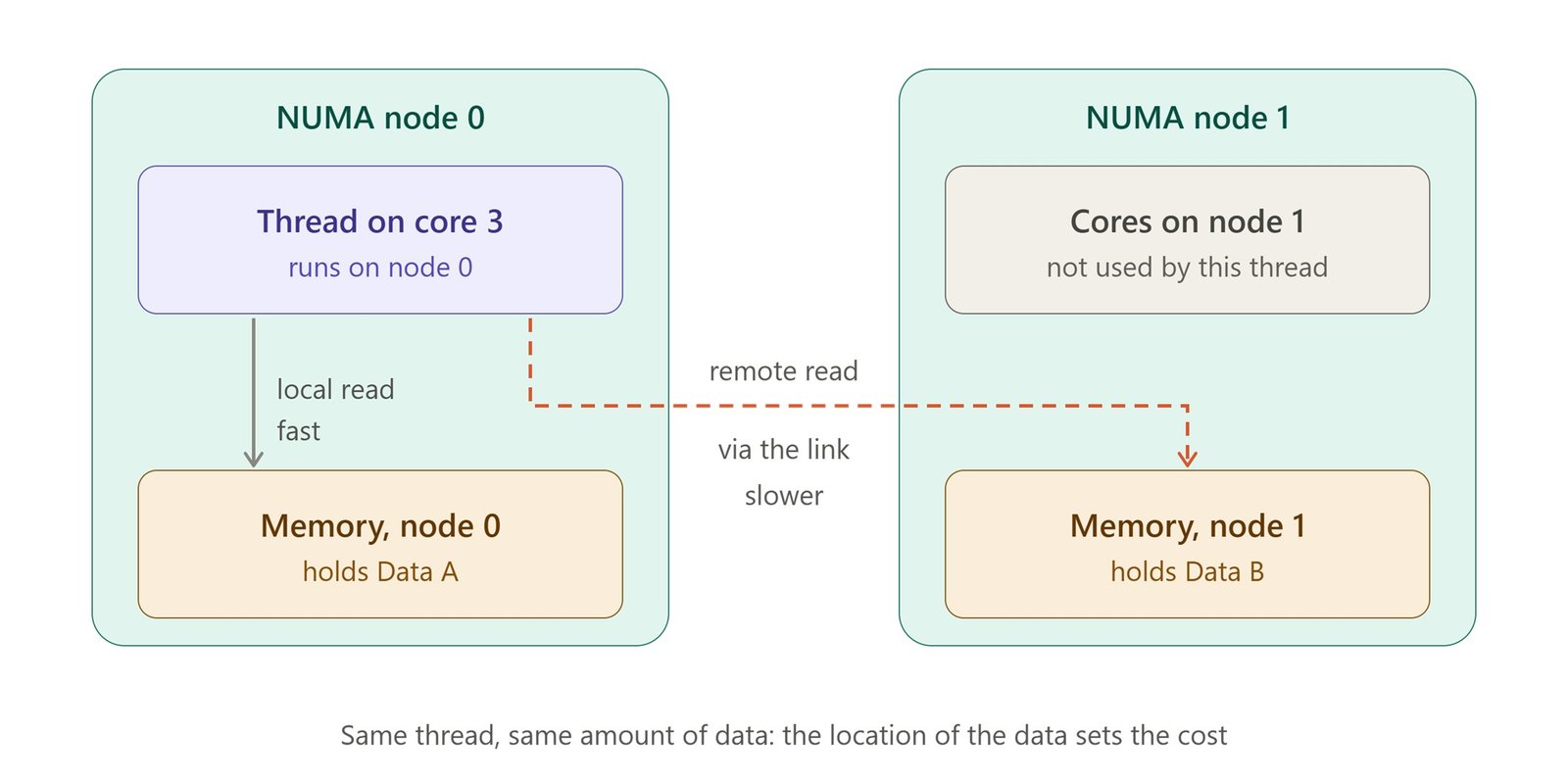
A server might have 512 GB of RAM in total, but that memory is split into pieces, for example 256 GB per node. Two services with identical memory footprints can perform very differently depending on whether their data sits in the same node as the cores that use it. Remote access typically costs noticeably more latency and offers less bandwidth than local access. The exact gap varies by hardware, and commonly lands around 1.5 to 2 times the local latency.
Important Point: Linux usually places a memory page on the node of the thread that first writes to it. If a master process loads a model while running on node 0, and workers are later scheduled on node 1, those workers read the weights remotely on every access. You can inspect the layout on a Linux server with numactl --hardware or lscpu. You can fix placement by pinning workers and their memory together, for example with numactl --cpunodebind=1 --membind=1.
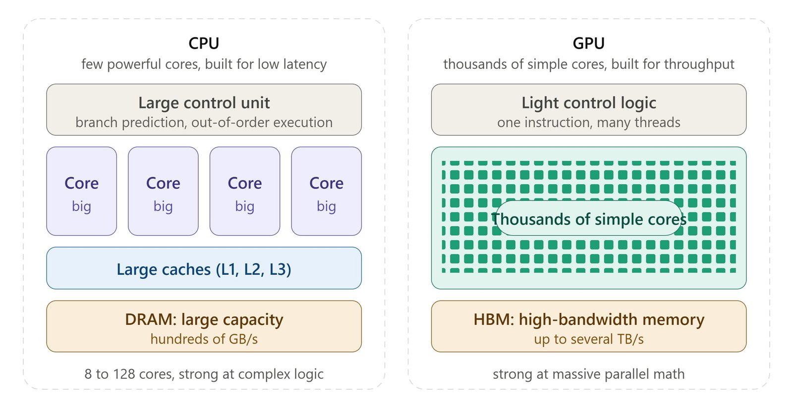
A GPU (Graphics Processing Unit) is a processor built to run a very large number of simple calculations at the same time. It was originally designed to render images, where millions of pixels can be computed independently. The same property turned out to suit neural networks, which are mostly large matrix multiplications. That is why GPUs now power AI training and inference. A CPU is the opposite kind of processor: it has a small number of powerful cores that handle complex, varied work one step at a time and finish each step quickly.
The diagram below compares how the two chips spend their silicon.
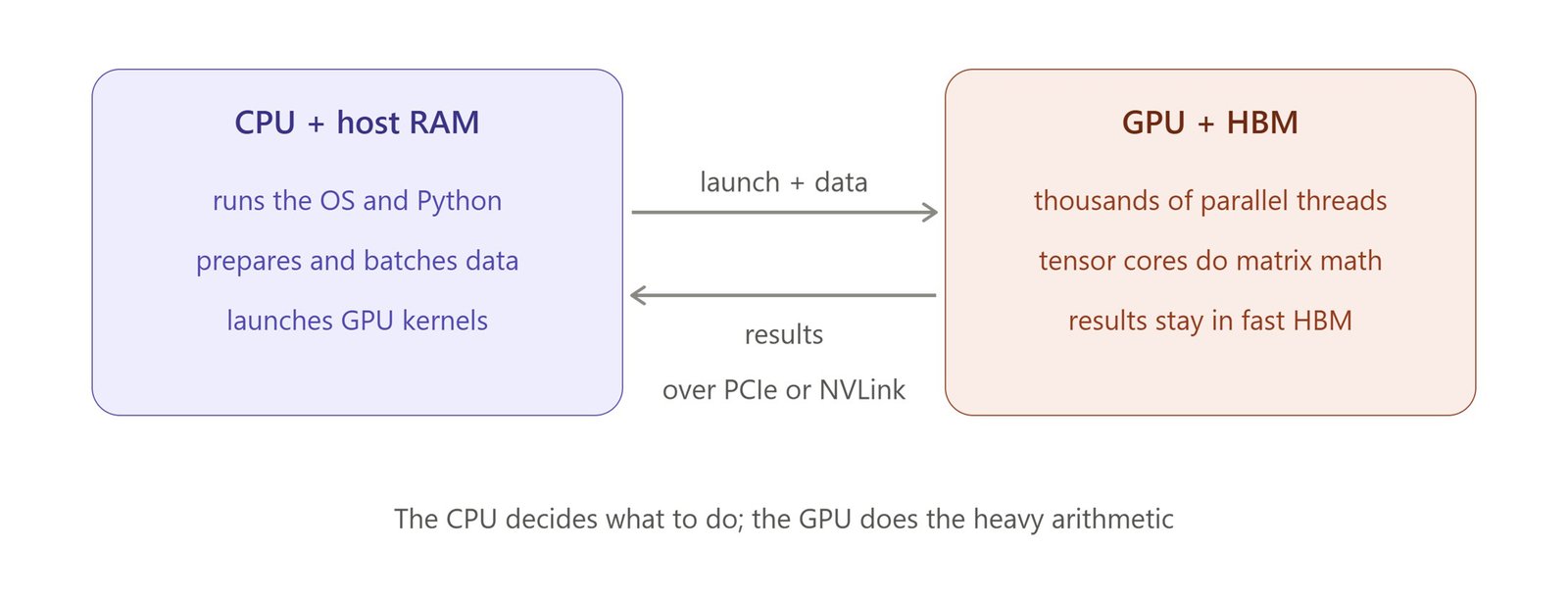
The CPU decides what to do; the GPU does the heavy arithmetic. The CPU side runs Python, so the interpreter, the GIL and NUMA placement shape how fast work reaches the GPU. The PCIe lanes carry the data and launch commands across, and the GPU's own memory holds the model weights while it computes. A fast GPU can sit idle if the CPU side feeds it too slowly, which is a common bottleneck in production AI serving.
HBM stands for High Bandwidth Memory. It is a type of DRAM designed to move data to a processor much faster than ordinary memory, and it is what most AI GPUs use as their main memory.
Ordinary memory modules sit in slots on the motherboard, far from the processor and connected by a relatively narrow bus. HBM takes a different approach. Several DRAM chips are stacked vertically, and the stack is mounted right beside the GPU die on a shared piece of silicon, so the connection can be extremely wide and extremely short.
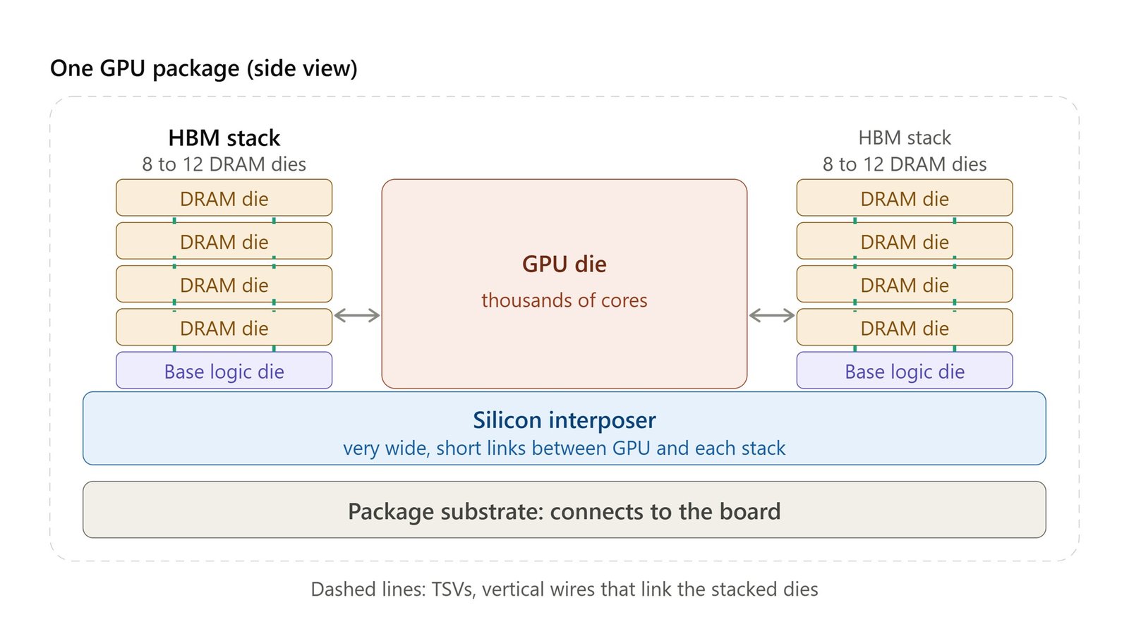
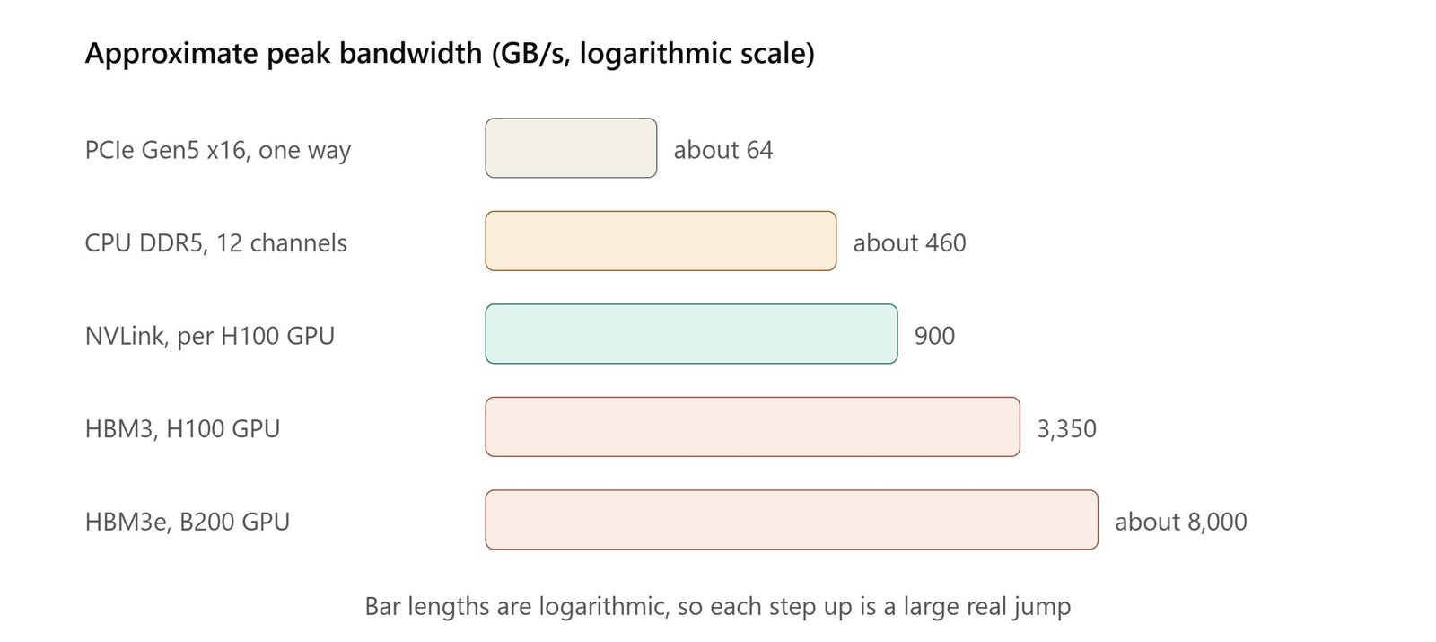
The figures above are approximate peak values and vary by product. The GPU's HBM delivers several times the bandwidth of the whole server's CPU memory, and orders of magnitude more than the PCIe link feeding it.
This matters for AI inference because generating each token requires reading essentially all of the model's weights from memory. That makes LLM inference limited largely by memory bandwidth rather than by raw arithmetic speed, so HBM bandwidth often sets the ceiling on tokens per second.
HBM has trade-offs too:
- Capacity is limited. A single GPU carries tens to a couple of hundred GB, such as 80 GB on an H100 and up to about 192 GB on a B200. That is far less than server DRAM, which can reach terabytes.
- It is expensive. Stacking dies and packaging them on an interposer is costly.
- It is not upgradeable. The memory is fixed inside the GPU package.
This is why the memory diagram in Figure 6 (Section. Memory: fork(), Copy-on-Write, and the Page-Sharing Trap) shows weights being copied from host RAM into HBM once per worker. The model must fit in HBM to run at full speed, and when it does not, techniques like tensor parallelism split it across several GPUs and use NVLink to keep them in step.
NVLink is NVIDIA's high-speed interconnect for connecting GPUs directly to each other. Without it, two GPUs in the same server can only exchange data over PCIe, usually by going through the CPU's PCIe root. NVLink gives them a dedicated, much faster path of their own.
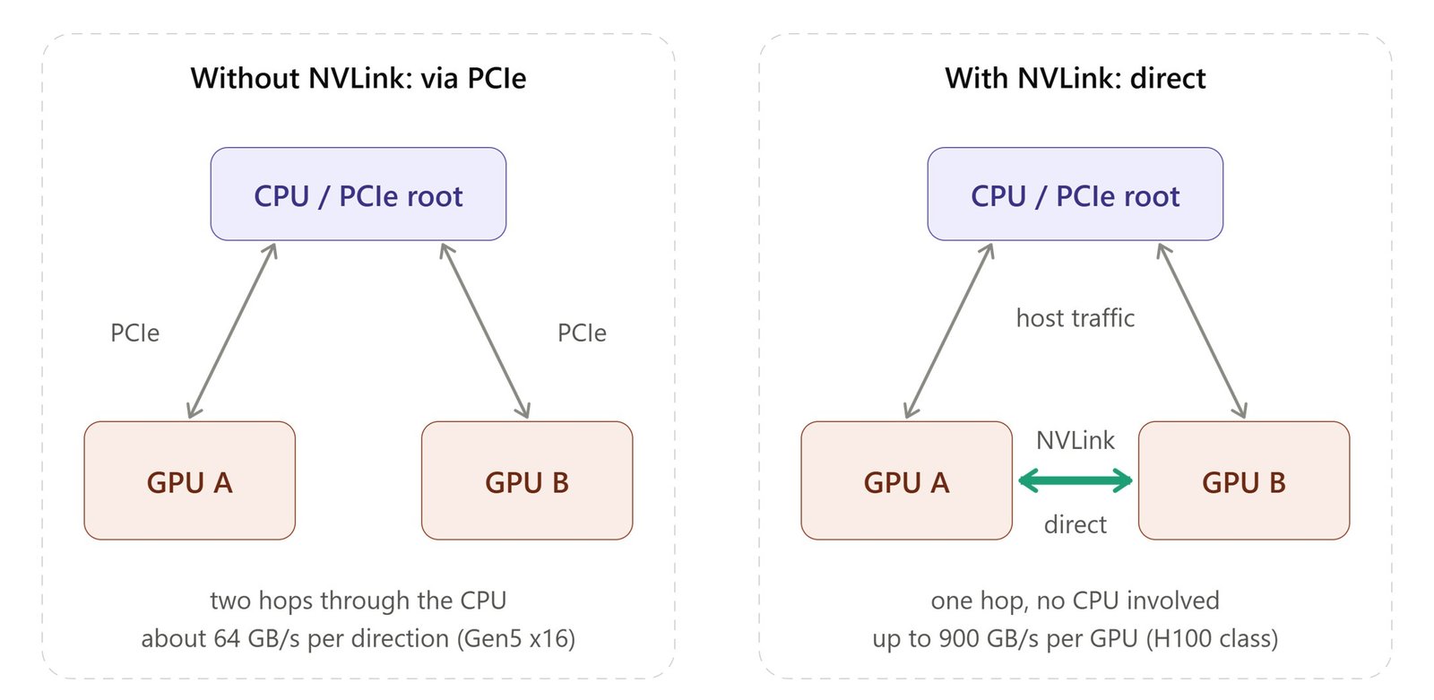
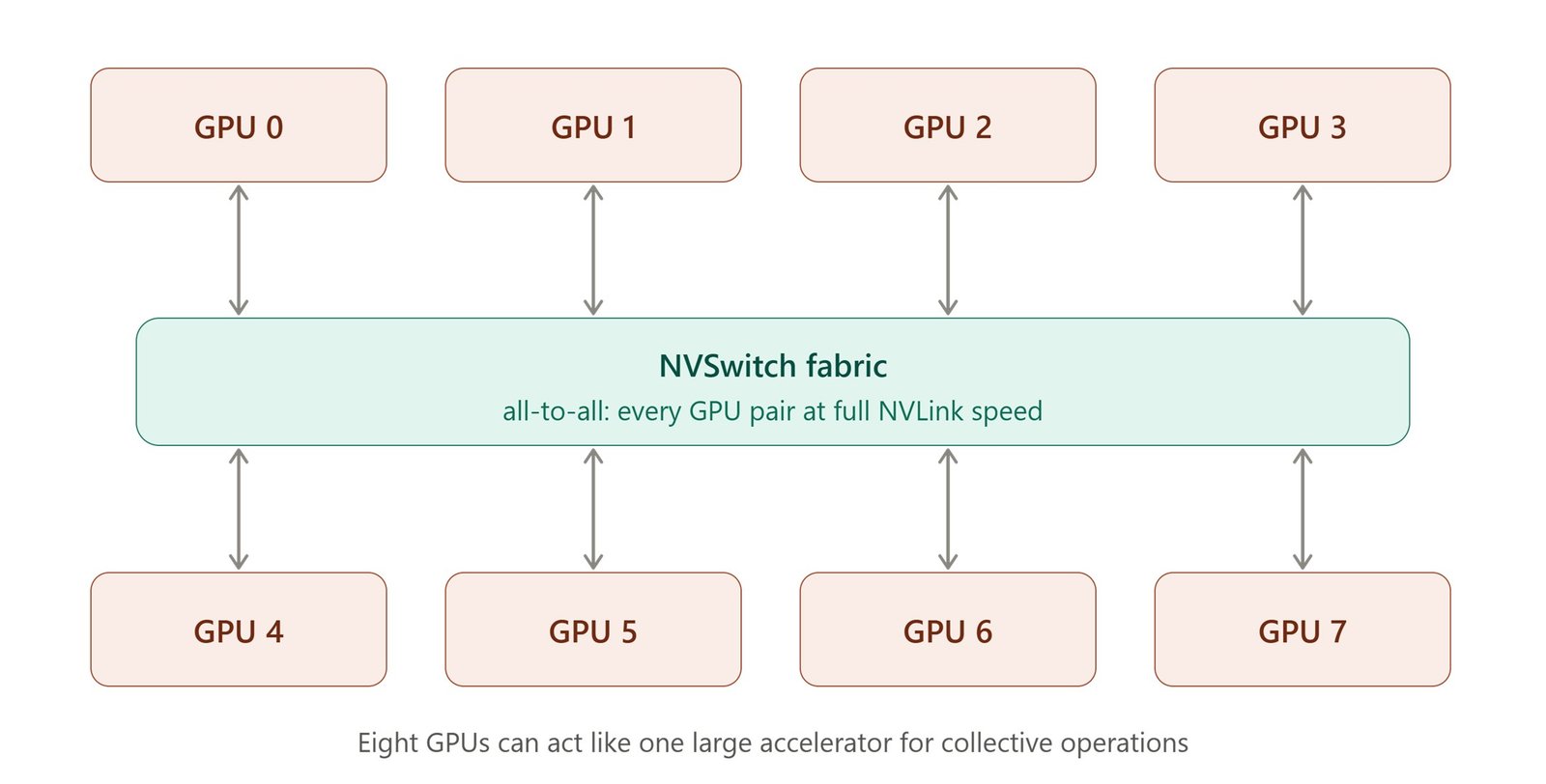
NVLink matters most when a model is too large for one GPU. Techniques such as tensor parallelism split each layer across several GPUs, and those GPUs must exchange intermediate results many times per token. Libraries such as NCCL perform these exchanges, and they run far faster over NVLink and NVSwitch than over PCIe. NVLink only works inside a node, so communication between servers uses a network such as InfiniBand or Ethernet instead.
In the hardware topology from this article, the two roles are separate. PCIe carries the CPU-to-GPU traffic, meaning data in and kernel launches. NVLink carries the GPU-to-GPU traffic, which is why it appears as its own link between the GPUs in Figure 1 (Section. Start with the Hardware: Topology Determines Placement).
WSGI stands for Web Server Gateway Interface. It is the traditional Python standard defined in PEP 3333 that allows web servers (like Gunicorn or Nginx) to communicate seamlessly with Python web applications and frameworks (like Django or Flask). It handles synchronous, one-way request-and-respo.
ASGI stands for Asynchronous Server Gateway Interface. It is the spiritual successor to WSGI, designed to provide a standard interface between async-capable Python web servers (like Uvicorn) and web frameworks (like FastAPI or modern Django). Unlike WSGI, it natively supports asynchronous features like long-polling, WebSockets, HTTP/2, and background tasks.
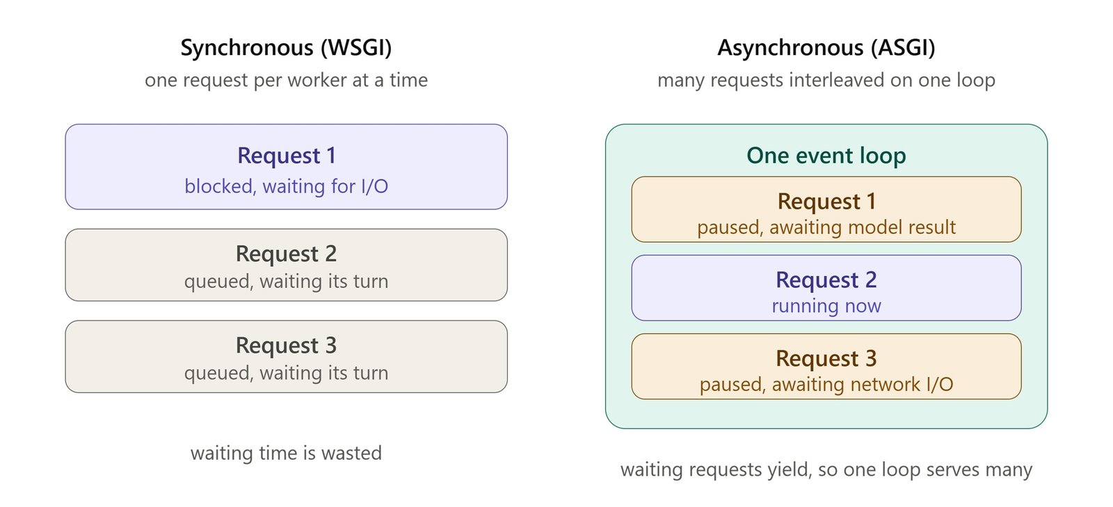
Gunicorn ("Green Unicorn") is a lightweight, production-ready Python WSGI HTTP Server for UNIX that manages and serves synchronous Python web applications. The master process acts as a manager that oversees worker processes, tracks their health, and restarts them automatically if they crash or time out. Worker processes execute isolated copies of the application code in memory to translate raw incoming HTTP requests into readable WSGI operations. It employs a pre-fork design where a single master process initializes the application and forks worker processes to handle high traffic concurrently. It supports synchronous workers by default, but allows alternative async configurations like Gevent or Eventlet for I/O-heavy workloads.
Uvicorn is a lightning-fast ASGI web server implementation for Python that bridges the gap between low-level network connections and high-performance asynchronous frameworks like FastAPI and Starlette. It handles thousands of concurrent client connections efficiently by executing non-blocking I/O operations through an event-driven loop. It works with any Python web framework that implements the ASGI standard, such as FastAPI, Starlette, and Django. It supports a built-in auto-reload flag for instant code refreshing during local development, and integrates seamlessly with Gunicorn worker configurations for stable production deployments.
An ASGI deployment means running a Python web application (typically a service that exposes an API over HTTP or WebSockets) written to the ASGI interface in production through an ASGI-capable server, usually with a process manager and a proxy around it. The schematic below shows the typical ASGI deployment stack.
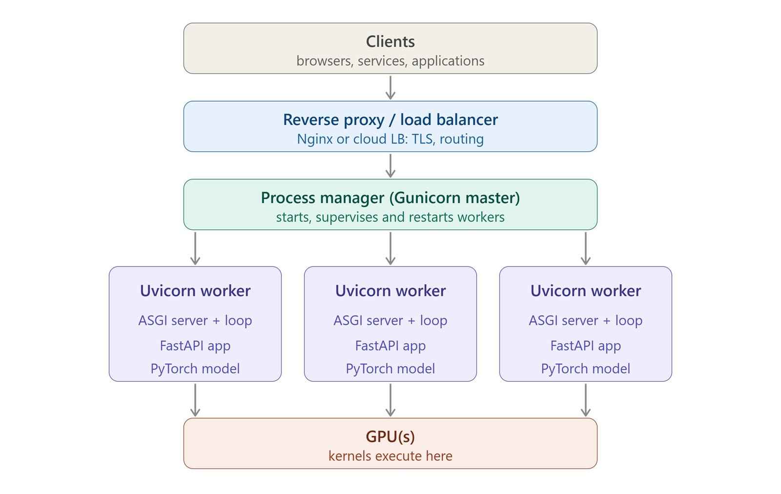
- Client Request: A browser or external application sends a request.
- Reverse Proxy (Nginx / Cloud LB): Handles encryption (TLS/SSL), serves static files, and routes incoming traffic to the application layer.
- Process Manager (Gunicorn Master): Instead of handling web traffic directly, the Gunicorn master process runs on a single thread. Its only job is to monitor system health, manage process lifecycles, and automatically restart crashed workers.
- Uvicorn Workers: Gunicorn forks multiple independent worker processes using Uvicorn's ASGI worker class. Each worker runs its own asynchronous event loop (uvloop), loads the FastAPI application, and manages incoming requests concurrently.
- GPU Execution: The FastAPI app inside the worker triggers heavy computations (like PyTorch model inferences), which are offloaded onto the system's GPU kernels.
An ASGI application is an async function that receives three arguments: a scope describing the connection, a receive channel for incoming events and a send channel for outgoing ones. Frameworks like FastAPI hide this contract, but every ASGI server and framework agrees on it.
async def app(scope, receive, send):
    ...  # read request events from receive(), write response events with send()
The caveat for AI workloads is that the event loop runs on a single thread under the GIL. While it is waiting, it serves other requests well. But if model code blocks it, for example a CPU-heavy tokenization step or a synchronous inference call that holds the thread, every other request on that worker stalls. That is why Figure 7 of this article (Section: Following One Request Through the Runtime) moves such work to thread pools, process pools and a dynamic batcher, and keeps the event loop free for accepting and streaming.
Introduction
Python is the working language of enterprise AI, yet it is often treated as a black box once an application leaves the developer's laptop. A service that handles ten requests per minute in development may be deployed onto a server with two CPU sockets, 64 cores, and four GPUs, with the expectation that the workload will scale with the available hardware. Sometimes it does. Often it does not. The reasons are rarely obvious from the application code alone.
The explanation lies in the runtime.
CPython is not an isolated execution environment. It is one layer in a larger system. The Python process runs under an operating system scheduler, which places runnable threads and processes onto CPU cores. Those cores operate within a memory hierarchy whose access costs vary significantly by locality. On multi-socket systems, memory may also be physically distributed across NUMA nodes, making the location of data as important as the amount of data. Within the interpreter itself, the execution model, memory-management mechanisms, and native extensions determine how effectively Python code can exploit the underlying machine.
For AI workloads, the picture becomes even more interesting. Frameworks such as PyTorch can move computation from Python into highly optimized native code and onto GPUs. A single Python request may therefore involve interpreter execution on one or more CPU cores, native computation in compiled libraries, memory movement across CPU and GPU boundaries, and parallel execution across thousands of GPU threads. The Python code is only the visible tip of a much larger execution system.
This article develops a runtime mental model for that system through seven schematic views, progressing from silicon and operating-system scheduling to the execution of a single inference request. Each view isolates one architectural idea: processor topology, core utilization, process and thread placement, memory locality, interpreter execution, native parallelism, and GPU execution. Taken together, they provide a practical way to reason about where a Python-based AI application actually runs, how much of the underlying hardware it can use, and why adding CPUs, cores, processes, or GPUs does not automatically produce linear performance gains.
The discussion assumes CPython 3.12 through 3.14, an ASGI deployment using a server such as Uvicorn or Gunicorn, an AI framework such as PyTorch, and GPU-accelerated inference. The objective is not to explain every implementation detail of CPython or every feature of a particular framework. It is to build the systems-level mental model required to make sound architecture, capacity-planning, deployment, and performance-engineering decisions for enterprise AI workloads.
Start with the Hardware: Topology Determines Placement
Python does not see the machine in the same way the machine is physically organized. A modern multi-socket server may contain two CPU sockets, with each socket providing its own CPU cores, shared last-level cache, and directly attached memory. Each socket and its associated memory form a NUMA node. Access to memory within the local NUMA node is generally lower latency and higher bandwidth than access to memory attached to another node. Under sustained load, remote memory traffic can also place additional pressure on the inter-socket fabric.
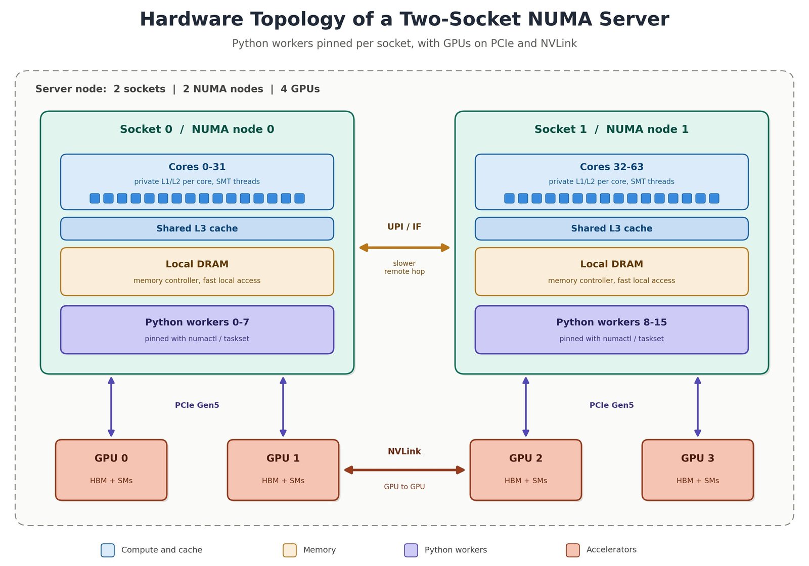
Figure 1: Hardware topology of a two-socket NUMA server with Python workers pinned per socket.
GPUs introduce another layer of topology. A GPU is connected to the host through a PCIe hierarchy, typically with a closer affinity to one CPU socket and its associated NUMA node. Depending on the platform, GPUs may also have high-bandwidth peer-to-peer links such as NVLink. Consequently, a worker running on one socket while frequently transferring data to a GPU with stronger affinity to another socket can incur additional latency and consume inter-socket or PCIe bandwidth. The exact cost depends on the server topology, PCIe configuration, workload, and data-transfer pattern.
The important architectural point is that CPython does not automatically optimize application placement according to this hardware topology. The operating system schedules processes and threads, while the application and its deployment configuration determine process placement, CPU affinity, memory policy, and GPU assignment.
This makes placement an architectural decision, not merely an operational tuning exercise. Tools such as numactl and taskset can constrain processes to specific CPUs or NUMA nodes, while the application and deployment configuration can establish affinity between workers, memory, and GPUs. When the workload is sensitive to memory locality or host-to-device transfers, aligning each worker with the resources it uses most heavily can reduce remote memory access, improve data locality, and make hardware utilization more predictable.
Figure 1 illustrates the basic principle: understand the physical topology first, then decide where the Python workers should run.
One Process, One Interpreter: The Anatomy of CPython
Every Python worker is an operating system process with its own virtual address space. Within that address space, several layers of execution and memory management coexist.
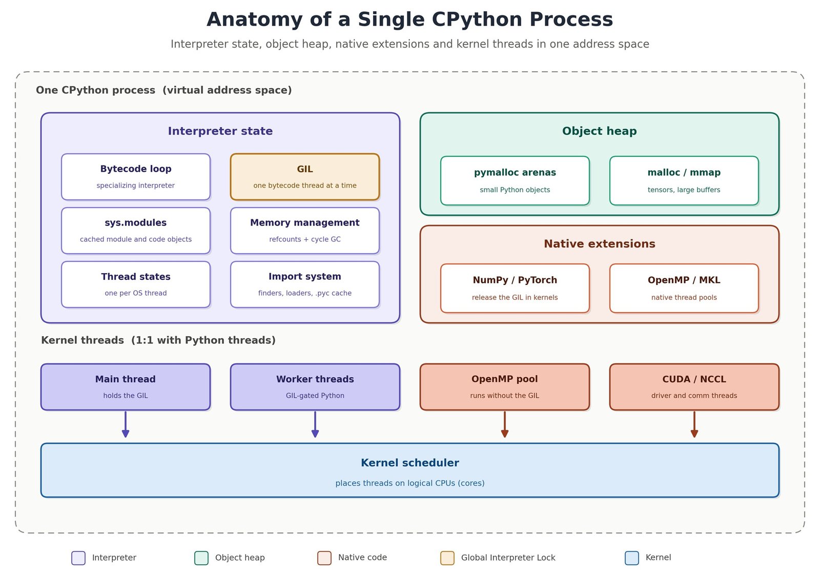
Figure 2: Anatomy of a single CPython process.
At the center is the CPython runtime. It maintains the interpreter state, executes Python bytecode, manages imported modules and Python objects, and maintains thread state for the threads associated with the interpreter. In traditional CPython builds, the Global Interpreter Lock (GIL) also governs access to the Python object model during bytecode execution. CPython's memory-management machinery includes reference counting and cyclic garbage collection, while its allocator uses mechanisms such as pymalloc for many small Python-object allocations and the platform allocator for larger allocations. Large application buffers, such as tensor storage, may ultimately be managed through native allocators and operating-system facilities such as mmap, depending on the library and allocation path.
The same process can also contain substantial amounts of native code. Libraries such as NumPy, PyTorch, OpenMP runtimes, and Intel oneMKL can execute compiled code outside the Python bytecode evaluation loop. They may release the GIL while performing computationally intensive operations and may create their own native worker threads. PyTorch, for example, can use CPU thread pools for parallel operators and can dispatch work to GPUs through its native runtime. These execution paths can therefore consume multiple CPU cores even though the application is controlled by a relatively small amount of Python code.
At the operating-system level, each process contains one or more OS threads. Python's threading model maps Python threads to native threads managed by the operating system. The OS scheduler then places those runnable threads on logical CPUs according to scheduling policy, CPU affinity, system load, and other constraints.
The key idea from Figure 2 is that a Python process is a hybrid execution environment. Python bytecode executes under the rules of the CPython runtime, while computationally intensive work can cross into native libraries that have their own execution models, thread pools, memory allocators, and accelerator runtimes.
That boundary is fundamental to understanding Python performance. A workload that spends most of its time executing Python bytecode is constrained by the interpreter's execution model. A workload that spends most of its time in native numerical kernels may scale across multiple CPU cores or GPUs even though only one Python thread is orchestrating the operation. The first step in explaining scaling behavior is therefore to identify where the actual work is being executed.
Loading the Application: The Startup Sequence
Startup is where an application's runtime architecture is quietly established. In a typical pre-fork deployment, a master process initializes the Python runtime, imports application modules, and may preload model weights into host memory. Once initialization reaches the appropriate point, the master calls fork() to create worker processes. Each worker then completes its own post-fork initialization, which may include creating an event loop, initializing application-specific resources, establishing its CUDA context, warming up the model, and reporting readiness.
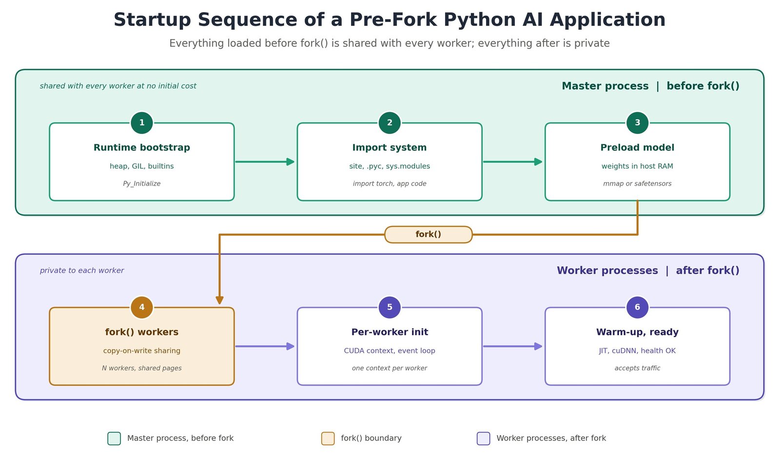
Figure 3: Startup sequence of a pre-fork Python AI application.
The position of the fork() boundary matters because it determines which resources exist before process duplication and which are created independently by each worker. Memory pages populated by the parent before fork() can initially be shared by the parent and its children through the operating system's copy-on-write mechanism. If a worker modifies one of those pages, the operating system creates a private copy for that worker. This makes preloading large read-mostly objects, such as model weights in host memory, potentially valuable for reducing aggregate memory consumption, although the actual savings depend on the allocator, memory access patterns, and subsequent mutations.
Accelerator state is different. CUDA contexts and other device-side runtime state should not be treated as fork-safe resources. In a conventional pre-fork architecture, CUDA initialization should therefore occur after the worker has been created. Each worker can then establish its own CUDA context and explicitly bind itself to the GPU assigned to that worker.
This distinction creates an important architectural boundary:
- Before
fork(): initialize resources that can safely participate in copy-on-write sharing, such as read-mostly host-memory data. - After
fork(): initialize resources that must belong to an individual worker, including event loops, worker-specific runtime state, and CUDA contexts.
The lesson from Figure 3 is that initialization order is part of the system architecture. The fork() boundary determines not only process creation, but also memory-sharing opportunities, resource ownership, accelerator initialization, and ultimately the runtime behavior of every worker.
Threads, the GIL, and Cores Over Time
In a traditional GIL-enabled CPython interpreter, only one thread can execute Python bytecode at a time. Multiple Python threads may be runnable simultaneously, but they take turns acquiring the GIL. CPython periodically evaluates whether another thread should be given an opportunity to run. The interpreter's thread-switching interval is configurable and defaults to five milliseconds in current CPython releases, but this value is not a guarantee that the GIL changes hands at precisely that interval.
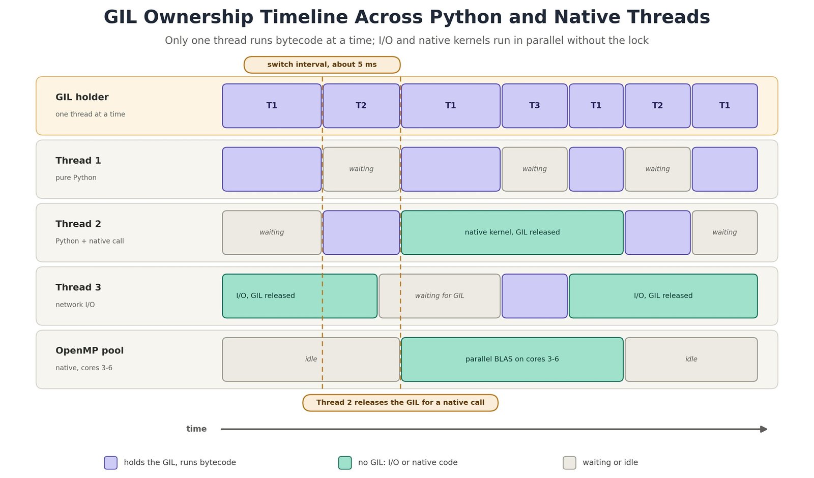
Figure 4: GIL ownership timeline across Python threads and native threads.
Figure 4 makes this behavior visible over time. The GIL lane shows which Python thread currently owns the lock, while the execution lanes show which threads are running, waiting, or blocked. The result is an important distinction between concurrency and parallelism: multiple Python threads can make progress concurrently, but within a single GIL-enabled interpreter, Python bytecode execution is serialized.
The more important question is what happens when a thread leaves the Python execution path. Threads blocked on operations such as network or disk I/O can release the GIL while they wait. Computational libraries implemented in native code can also release the GIL around operations that do not require access to Python objects. NumPy, PyTorch, and BLAS implementations commonly use this model for computationally intensive operations, although the exact behavior depends on the operation and library implementation.
Once execution moves into native code, a different form of parallelism can emerge. A single Python thread may invoke a native numerical kernel that creates or uses its own worker threads. An OpenMP or BLAS runtime, for example, may distribute computation across multiple CPU cores while the Python interpreter is free to schedule other work. In GPU workloads, the native framework may instead enqueue operations on a GPU, allowing the CPU and accelerator to execute different portions of the workload concurrently.
Figure 4 therefore corrects a common misconception: the GIL does not make a Python process single-core. It serializes Python bytecode execution within a GIL-enabled interpreter.
The practical consequence is workload dependent. Applications dominated by Python-level computation are constrained by this serialization within each interpreter. Applications dominated by I/O can achieve substantial concurrency with threads, while applications that spend most of their time in native numerical kernels can exploit multiple CPU cores or GPUs despite being orchestrated by Python.
Four Ways to Use Many Cores
Python provides several ways to exploit parallel hardware, but they differ substantially in how they balance isolation, memory sharing, interpreter independence, and ecosystem compatibility.
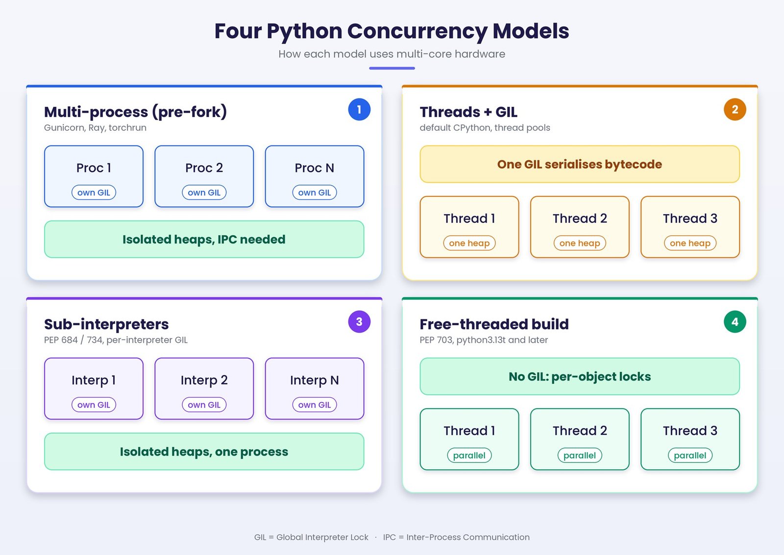
Figure 5: Four Python concurrency models on multi-core hardware.
Multi-process execution gives each worker its own operating-system process, virtual address space, Python interpreter, and object heap. Each process can execute Python bytecode independently, allowing multiple workers to run Python code in parallel across different CPU cores. Processes also provide strong fault and resource isolation. The trade-off is higher memory consumption, process-management overhead, and the need for explicit inter-process communication when workers must exchange state.
Threads within a process provide a lighter-weight concurrency model. Threads share the process address space and Python objects, making communication and resource sharing relatively inexpensive. In a GIL-enabled CPython interpreter, however, only one thread at a time can execute Python bytecode. Threads can still provide substantial concurrency for I/O-bound workloads and for operations that spend most of their execution time in native code that releases the GIL.
Sub-interpreters provide another point in the design space. CPython 3.12 introduced a per-interpreter GIL, allowing different sub-interpreters within the same process to have independent interpreter locks. Python 3.14 adds a standard-library API for creating and managing sub-interpreters. Each interpreter has its own Python runtime state and object namespace, while the interpreters remain within the same operating-system process. This can provide parallel Python execution with a different isolation and sharing model from either threads or separate processes. Extension-module compatibility and the rules governing objects shared between interpreters remain important considerations.
Free-threaded CPython takes a different approach by removing the GIL from a specialized CPython build and replacing its global serialization point with finer-grained synchronization mechanisms. Python 3.13 introduced experimental free-threaded builds, and Python 3.14 continues their development and support. With a compatible application and extension stack, multiple threads can execute Python code concurrently within the same interpreter, potentially allowing a single process to use multiple CPU cores for Python-level work. The trade-off is that the application and its native dependencies must be compatible with the free-threaded execution model, and performance characteristics can differ from conventional GIL-enabled CPython.
Figure 5 therefore represents more than four programming techniques. These models occupy different positions along two fundamental architectural dimensions: isolation and sharing. Processes provide stronger isolation with separate address spaces. Threads provide extensive sharing with minimal isolation. Sub-interpreters provide isolated interpreter state within a shared process. Free-threaded execution maximizes concurrent access to shared process memory while removing the GIL as the primary serialization mechanism.
For production AI systems, the practical choice is often layered rather than exclusive. A deployment may use multiple Python processes to distribute requests across NUMA nodes or GPUs, while each process relies on native thread pools for CPU-intensive operations and GPU runtimes for accelerator execution. Sub-interpreters and free-threaded CPython expand the design space, but their suitability depends on the Python version, framework, native extensions, deployment model, and operational requirements of the workload.
The architectural question is therefore not simply, "How do I use all the cores?" It is, "Which execution model should own each layer of parallelism?"
Memory: fork(), Copy-on-Write, and the Page-Sharing Trap
After fork(), worker processes do not immediately receive independent copies of the parent's address space. The operating system creates a new process with its own page tables, while the parent and child initially reference the same physical memory pages. Those pages remain shared until one of the processes attempts to modify them. When a write occurs, the operating system creates a private copy of the affected page for the writing process. This copy-on-write mechanism is what makes preloading large, read-mostly data structures before fork() potentially attractive for memory efficiency.
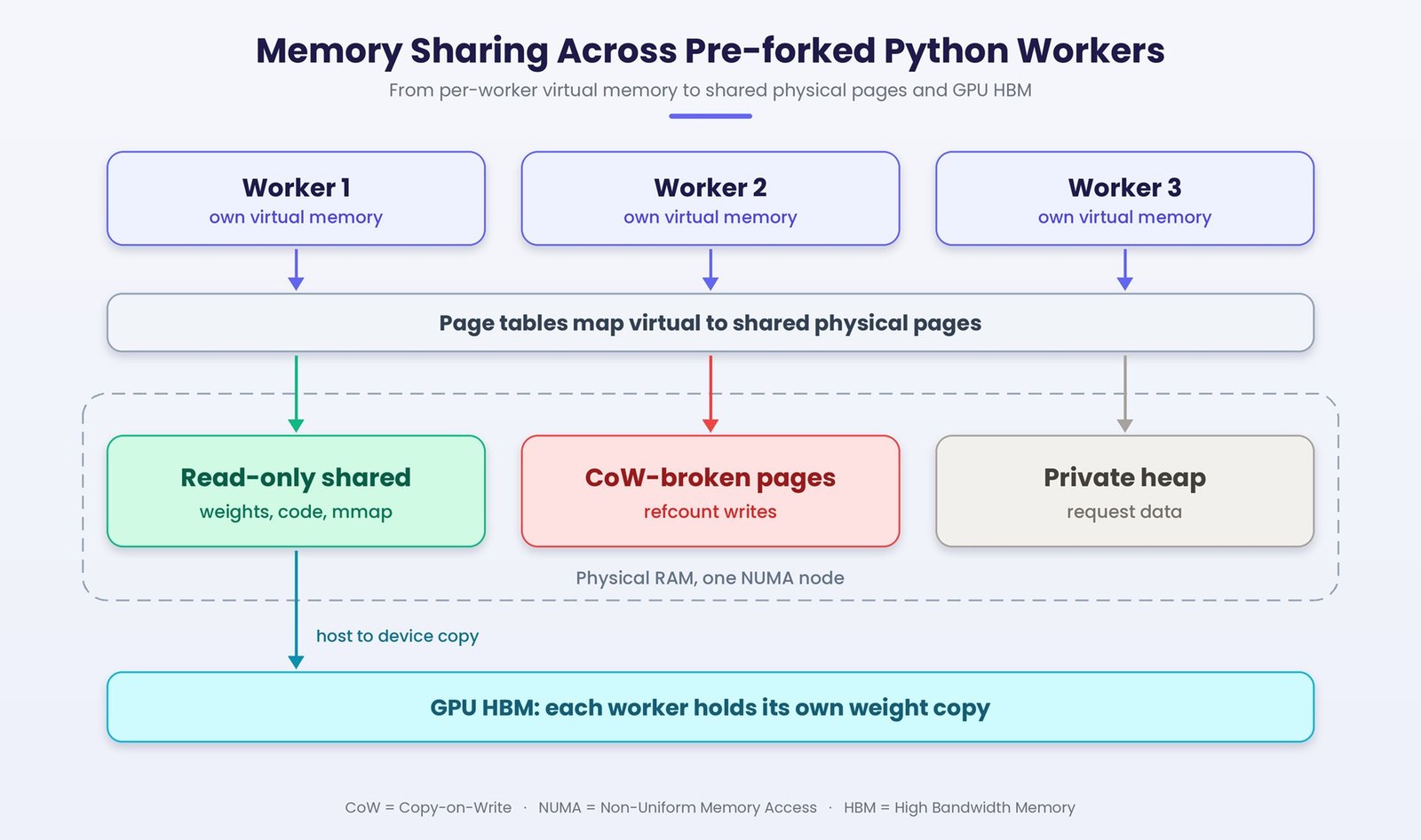
Figure 6: Memory sharing across pre-forked Python workers.
CPython introduces an important complication. Python objects contain interpreter-managed metadata, and operations that appear logically read-only can still modify that metadata. In particular, reference-count updates can write to object headers. If those headers reside on pages shared with other workers, such writes can trigger copy-on-write faults and cause additional physical pages to become private to the worker. The result is that the memory footprint of pre-forked workers can grow even when the application appears to be reading rather than modifying a large in-memory object.
Figure 6 separates the resulting physical memory into three conceptual populations. The first consists of pages that remain genuinely shared, such as read-only code and data that workers do not modify. The second consists of pages that were initially shared but became private after a worker modified them, including pages affected by interpreter-managed object metadata. The third consists of memory that was private to a worker from the beginning, including worker-specific application state and allocations performed after the fork.
GPU memory introduces another boundary. A model loaded into host memory is not automatically shared as a single physical allocation across GPU contexts. When multiple workers independently load or materialize the model on a GPU, each worker can consume its own allocation in device memory. Consequently, a deployment that appears memory-efficient in host RAM can still consume substantial GPU memory as the number of workers increases.
Several techniques can reduce unnecessary memory amplification. gc.freeze() can reduce certain forms of post-fork garbage-collector activity for long-lived objects. Memory-mapping immutable data can provide a more explicit mechanism for sharing read-only data between processes. Formats such as safetensors can support memory-efficient, structured model loading, particularly when combined with appropriate loading strategies. Worker recycling can also place an upper bound on memory growth caused by fragmentation, allocator behavior, or application-level leaks, although it does not solve the underlying copy-on-write mechanism.
The key lesson from Figure 6 is that virtual memory sharing is not the same as permanent physical memory sharing. A pre-fork architecture can begin with a highly shared address space and gradually converge toward substantially higher per-worker memory consumption as workers touch and modify shared pages. Understanding which pages are genuinely immutable, which are vulnerable to copy-on-write, and which must be private is essential when sizing a multi-worker Python AI deployment.
Following One Request Through the Runtime
The final view follows a single inference request through the runtime. The request first reaches the server's event-loop thread, where the application accepts and parses the request and performs the initial Python-level processing. This work executes under the GIL in a GIL-enabled CPython interpreter. CPU-intensive preparation, such as tokenization or preprocessing, may then be delegated to a thread pool or process pool so that it does not unnecessarily block the event loop.
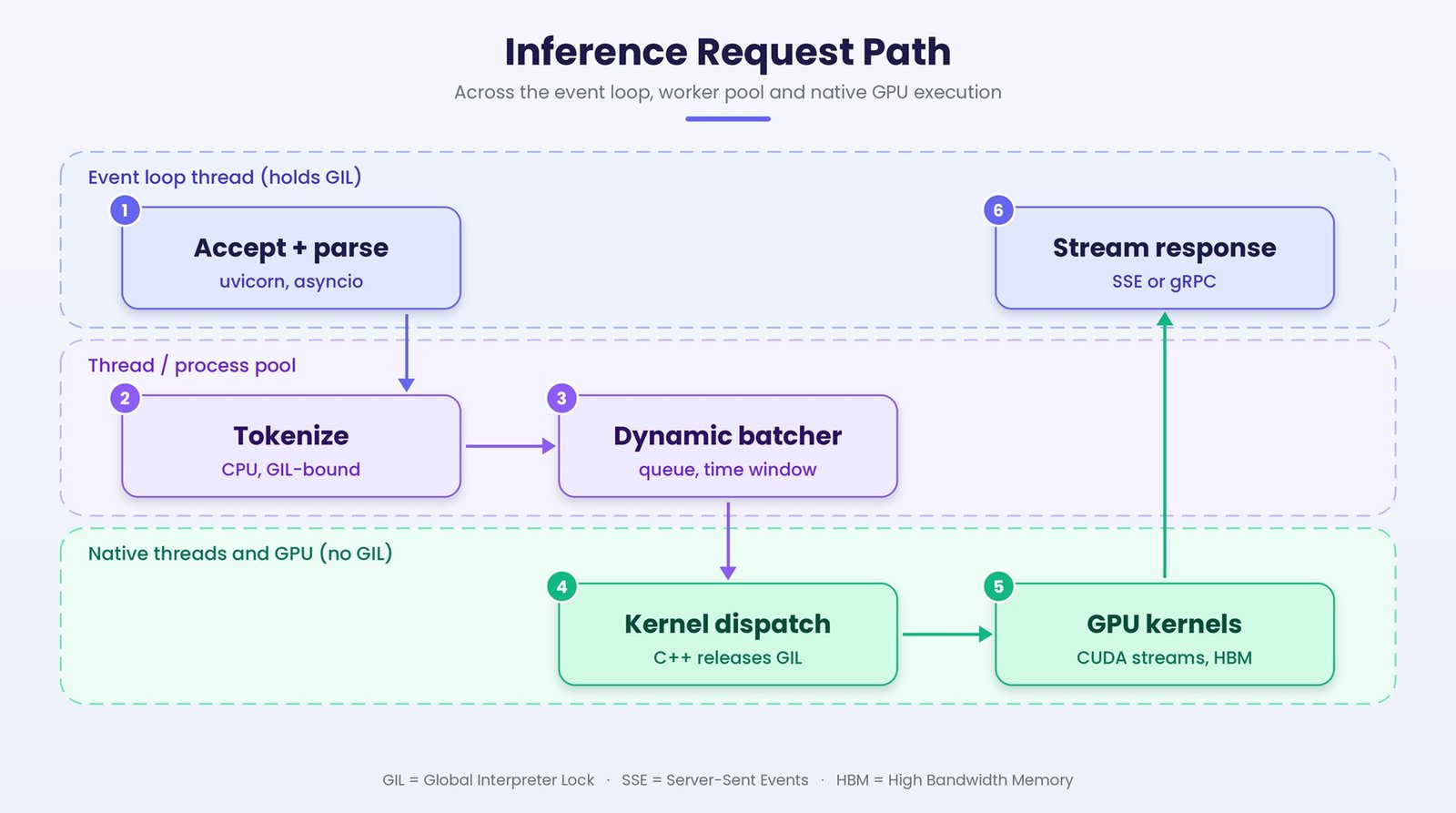
Figure 7: Inference request path across the event loop, worker pool, and native GPU execution.
A dynamic batcher may collect multiple requests over a short interval and combine them into a larger inference operation. The AI framework then crosses the Python-to-native boundary, invoking compiled kernels and runtime libraries. These operations can release the GIL while CPU-side native code executes in parallel or while work is submitted to the GPU. The GPU subsequently performs the model computation, often asynchronously from the CPU. Once the required results are available, control returns to the application, which performs any final post-processing and streams the response back to the client.
Figure 7 is organized into three conceptual execution lanes because the request crosses three different runtime domains. The first lane is dominated by Python application execution and event-loop scheduling. The second is dominated by CPU-side preparation, batching, and native execution. The third is dominated by accelerator execution. The GIL is relevant to Python-level execution in the first lane, may be temporarily released during native execution in the second lane, and is not involved in the GPU's execution of device kernels.
This separation provides a useful way to reason about latency. If Python-level tokenization blocks the event loop, requests can queue before they reach the model. If a CPU worker pool is saturated, requests can wait before inference begins. If the batcher is starved, GPU utilization can remain low even when accelerator capacity is available. Conversely, once the workload reaches the GPU, the dominant constraints may shift to device compute, device memory, host-to-device transfers, synchronization, or insufficient batching.
The important tuning principle is therefore to identify where the request is spending time before moving work across execution boundaries. Improving the event loop will not solve a GPU bottleneck, and adding GPU capacity will not solve a CPU-bound tokenizer that prevents requests from reaching the GPU efficiently.
Operating Considerations
Three practical concerns cut across all seven views.
First, container CPU visibility must be treated carefully. The number returned by os.cpu_count() reflects what the Python runtime reports as available CPUs and should not be assumed to represent the container's effective CPU entitlement in every deployment configuration. Depending on the Python version, operating-system configuration, and container runtime, CPU affinity and cgroup limits can produce different views of available capacity. Worker counts and native thread pools should therefore be configured with the container's actual CPU quota or affinity in mind rather than blindly sizing them from the host's physical topology.
Second, native parallelism must be accounted for alongside Python workers. A Python worker may invoke OpenMP, BLAS, MKL, PyTorch, or other native runtimes that create additional threads. If several workers each create large native thread pools, the combined runnable-thread count can greatly exceed the CPUs allocated to the container or NUMA node. The resulting oversubscription can increase context switching, cache contention, memory bandwidth pressure, and CPU throttling. Settings such as OMP_NUM_THREADS and MKL_NUM_THREADS, together with the application server's worker count, should therefore be treated as a coordinated capacity-planning decision.
There is no universal rule that the product of Python workers and native threads must equal or remain below the number of physical cores. The appropriate configuration depends on whether the workload is CPU-bound, I/O-bound, latency-sensitive, memory-bandwidth-bound, or primarily GPU-bound. The goal is to provide enough parallelism to keep the hardware busy without creating unnecessary contention.
Third, training introduces another process topology. Distributed training launchers such as torchrun commonly create one process per GPU. Each process then has its own Python interpreter and runtime state, while GPU communication may be coordinated through libraries such as NCCL. DataLoader workers, CPU preprocessing, communication threads, and native framework thread pools add further CPU consumers. The same process-level mental model therefore applies to training, but the resource graph becomes more complex because CPU placement, GPU affinity, inter-GPU communication, and input-pipeline throughput must all be considered together.
Across all seven figures, the recurring principle is the same: Python is only one layer of the execution system. To understand the performance of an enterprise AI application, you must follow the workload across processes, threads, memory, native libraries, operating-system scheduling, and accelerators. Once those execution boundaries are visible, CPU utilization, memory growth, GPU utilization, queueing, and latency become architectural behaviors that can be reasoned about rather than mysterious runtime effects.
Conclusion
The performance of an enterprise Python AI application is the result of decisions and interactions across multiple layers of the execution stack. Hardware topology determines where CPUs, memory, and GPUs are located. The operating system determines where processes and threads execute. The Python runtime determines how Python-level work is scheduled and synchronized. The memory model influences how much physical RAM a fleet of workers ultimately consumes. Native libraries introduce their own forms of parallelism. The request path determines where work queues, waits, and latency accumulate.
The seven schematics in this article are designed to be read as one continuous model, progressing from physical topology to the execution of a single request. Together, they provide a disciplined way to investigate performance problems by asking the right question at the right layer:
- Is the workload correctly placed relative to CPU, memory, NUMA, and GPU topology?
- Is the work executing as Python bytecode, native code, or GPU kernels?
- Is the GIL limiting Python-level concurrency?
- Are pre-forked memory pages remaining shared, or are copy-on-write effects increasing the physical memory footprint?
- Is the selected concurrency model appropriate for the workload?
- Are native thread pools and worker processes creating unnecessary oversubscription?
- Where does a request actually spend its time?
These questions turn Python performance from an application-level mystery into a systems-level analysis problem. They help architects size infrastructure more accurately, engineers avoid unnecessary contention and oversubscription, and operations teams trace production latency and memory behavior to the layer where the constraint actually exists.
The specific mechanisms will continue to evolve. Sub-interpreters, free-threaded CPython, increasingly sophisticated native runtimes, and new accelerator architectures will expand the ways Python applications can occupy modern hardware. The fundamental method, however, remains stable: understand the topology, identify the execution domain, trace the resource ownership, and follow the workload through the entire runtime stack.
That is the mental model required to think about Python not simply as a programming language, but as a runtime that occupies a multi-processor, multi-core, and increasingly heterogeneous machine.
✍️ About the Author
Sanjoy Kumar Malik — Principal AI Architect, Enterprise AI Strategist, and Senior Engineering & Technology Leader with 20+ years of corporate IT experience and a broader 27+ year professional journey, spanning Enterprise Architecture, software architecture, cloud-native systems, engineering leadership, and AI architecture. He is a TOGAF 10 Certified Enterprise Architecture Practitioner and AWS Certified Solutions Architect – Professional.
Sanjoy focuses on translating business strategy and AI opportunity into coherent enterprise architecture and scalable engineering execution. He works at the intersection of business, technology, architecture, and AI, helping organizations establish the architectural foundations, technology capabilities, and engineering systems required to turn AI initiatives into production-grade, scalable, governed, and economically sustainable enterprise capabilities.
He is the creator of The 28-Category AI Architecture Decision Framework (28-CAADF), a systematic approach to making AI architecture decisions in an era where intelligence itself is becoming an architectural capability.