Thinking in Hardware Infrastructure for Production LLM, GenAI & Agentic AI Systems

Publication Date: September 28, 2026 Last Updated: September 28, 2026

Introduction

Building a production-grade LLM, GenAI, or Agentic AI system is not simply a matter of selecting a powerful GPU, deploying a model, and exposing an API.

The moment an AI application moves from experimentation into production, infrastructure becomes an architectural concern.

A model that performs well in a development environment can behave very differently under real enterprise workloads. User concurrency increases. Context windows grow. Agentic workflows generate multiple model calls for a single business task. Retrieval introduces additional compute, storage, and network demands. Long-running conversations increase KV-cache pressure. Peak traffic creates contention. Availability requirements introduce redundancy. Security and governance introduce additional constraints. And suddenly, the question is no longer:

“Which GPU should we use?”

The real architectural question becomes:

“What infrastructure is required to execute this AI workload reliably, at the required scale, latency, quality, availability, and cost?”

Answering that question requires a different way of thinking.

Instead of starting with hardware specifications, start with the business workload. Understand the business process, users, transaction or data volumes, growth expectations, and the role AI plays within that process. Translate those business characteristics into the actual AI workload: inference, RAG, agentic execution, embedding, reranking, batch processing, fine-tuning, or a combination of these.

Then establish the latency and quality targets that the AI system must satisfy.

Only after these constraints are understood does it make sense to examine how the chosen model behaves, how many tokens it processes, how much memory it consumes, how much compute it requires, how much data must move across the network, and how much storage the overall system needs.

The fundamental reasoning chain becomes:

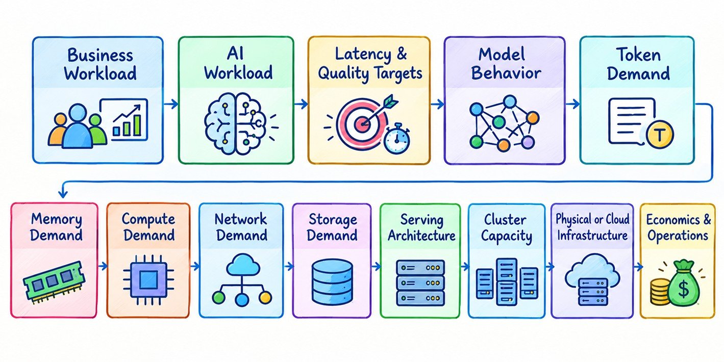
This chain is the foundation of hardware infrastructure thinking for production AI.

It is particularly important for Agentic AI, where the relationship between business requests and infrastructure demand is no longer one-to-one. A single user request may trigger planning, multiple LLM invocations, retrieval operations, tool calls, observations, retries, state updates, and additional reasoning steps. The infrastructure therefore needs to be sized not merely for requests per second, but for the entire AI execution trajectory generated by those requests.

The same principle applies to RAG, multimodal AI, batch inference, fine-tuning, and other enterprise AI workloads. Each workload produces a different computational and infrastructure profile.

This framework is therefore not intended to be a catalog of GPUs, servers, or cloud instance types. It is a thinking framework for deriving infrastructure from workload characteristics.

The central principle is:

Do not choose the hardware first and then try to fit the AI workload into it. Start with the workload and derive the infrastructure.

That shift—from hardware selection to infrastructure reasoning—is what enables an architect to design AI systems that are not only capable of running a model, but capable of running it reliably, efficiently, predictably, and economically in production.

With that foundation established, the first question is not “Which GPU do we need?”

It is:

What exactly is the AI workload we are trying to run?

Before jumping into AI Workload, we will start with Business Workload.

Section Map

Section #	Section Name	Section Purpose
1	Start With the Business Workload	Establish the business activity that the AI system must support, including volume, frequency, concurrency, seasonality, and growth. Infrastructure begins with workload, not hardware.
2	Translate Business Workload Into AI Workload	Convert business activity into the actual AI computation it generates, including inference, RAG, agentic execution, embeddings, reranking, batch processing, and other AI workloads.
3	Define Latency & Quality Targets	Establish the performance and quality boundaries that the infrastructure must satisfy, including latency, throughput, availability, accuracy, and task-level objectives.
4	Understand Model Behavior	Examine how model architecture, parameter count, context length, attention mechanism, precision, quantization, and generation characteristics influence infrastructure demand.
5	Understand Token Demand	Quantify input and output token consumption across requests, model calls, RAG context, and agentic trajectories to establish the fundamental workload volume.
6	Derive Memory Demand	Translate model weights, KV cache, activations, runtime buffers, communication buffers, and operational headroom into accelerator and system memory requirements.
7	Derive Compute Demand	Determine the CPU and accelerator computation required to execute inference, preprocessing, orchestration, retrieval, embeddings, reranking, and other AI workloads at the required scale.
8	Derive Network Demand	Determine network requirements for application traffic, data movement, distributed inference, and accelerator-to-accelerator communication, where the network can become part of the compute path.
9	Derive Storage Demand	Identify storage requirements for models, datasets, documents, embeddings, indexes, checkpoints, caches, temporary data, and persistent enterprise AI state.
10	Design the Serving Architecture	Translate workload characteristics into an inference-serving architecture covering routing, batching, caching, model pools, scheduling, replicas, and request management.
11	Design the Cluster Capacity	Convert workload demand into cluster-level capacity, accounting for peak traffic, concurrency, growth, resilience, utilization, and operational headroom.
12	Validate With Workload-Specific Benchmarking	Replace theoretical estimates with empirical measurements using the actual model, precision, context, concurrency, batching, and latency requirements.
13	Design the Physical or Cloud Infrastructure	Map validated capacity requirements to physical servers, accelerators, memory, networking, storage, cloud instances, managed services, regions, and availability zones.
14	Design for Reliability and Resilience	Engineer the infrastructure to tolerate failures across GPUs, nodes, racks, networks, storage, models, dependencies, and regions while maintaining required service levels.
15	Design Autoscaling and Scheduling	Align infrastructure capacity dynamically with changing workloads through autoscaling, workload scheduling, queue management, priority handling, and resource allocation.
16	Design Agentic Infrastructure	Extend infrastructure thinking from individual inference requests to complete agent execution trajectories involving planning, multiple model calls, tools, retrieval, state, retries, and loops.
17	Design RAG Infrastructure	Treat retrieval-augmented generation as a distributed workload spanning ingestion, chunking, embeddings, indexing, retrieval, reranking, context construction, and generation.
18	Design Observability	Establish visibility across infrastructure, inference, workload, and AI quality so that capacity, performance, failures, cost, and model behavior can be continuously understood.
19	Design Security and Isolation	Protect models, data, workloads, tenants, and infrastructure through identity, access control, network isolation, encryption, workload boundaries, secrets management, and governance controls.
20	Design Economics & Operations	Connect infrastructure architecture to operational reality by analyzing total cost, utilization, unit economics, platform operations, power, cooling, licensing, and engineering overhead.
21	Close the Loop With Continuous Capacity Planning	Establish a continuous cycle of measurement, analysis, benchmarking, optimization, resizing, and forecasting as workload and model behavior evolve.
22	The Complete Hardware Infrastructure Mental Model	Bring the entire reasoning chain together, showing how business workload ultimately drives AI workload, resource demand, serving architecture, infrastructure capacity, and economics.

Start With the Business Workload

Every hardware decision for an AI system is ultimately a decision about a business workload.

Yet many organizations begin at the opposite end. They select accelerators, negotiate cloud commitments, compare instance types, or benchmark models before they can answer a more fundamental question: How much work must the system actually perform, and under what conditions?

That inversion is expensive.

It produces clusters that remain underutilized for much of the day, capacity that cannot absorb predictable peaks, and architectures that are optimized for benchmark performance rather than business outcomes. The problem is rarely that the hardware is incapable. The problem is that the workload was never defined precisely enough to determine what the hardware needed to do.

The discipline is simple to state and difficult to practice:

Before choosing the model, understand the business workload the AI system must support.

Infrastructure should emerge from that understanding, not precede it.

The Questions That Define the Workload

Treat workload definition as an engineering intake, not a business questionnaire. Complete it with the business owner before discussing accelerators, instance families, cluster sizes, or deployment topology.

Purpose and Criticality

Start with the role AI plays in the business process.

What business process is being supported?
What business outcome does the AI system produce?
Which parts of the process are business-critical?
What is the operational or financial consequence of an outage, delay, or degraded response?
Which interactions are real-time, where a person or system is waiting for the answer?
Which workloads are batch, where results can arrive minutes or hours later?

These questions establish the service characteristics the infrastructure must support. A model serving a revenue-generating customer interaction has a different infrastructure requirement from a model processing an overnight analytics workload.

Scale and Volume

Next, quantify the amount of business activity.

How many users, customers, employees, or systems generate demand?
How many transactions, documents, conversations, events, or workflows occur?
What is the volume per hour, day, week, and month?
What proportion of that volume actually requires AI?

That last question is particularly important. Business volume is not necessarily AI volume. A business may process one million transactions a month while only a fraction of those transactions require model inference.

Shape and Growth

Finally, understand how the workload behaves over time.

What is the average workload?
What is the peak workload?
How frequently do peaks occur?
How long do they last?
How does demand vary across the day, week, month, and fiscal year?
What growth is expected over the planning horizon?
What business factors will drive that growth?

These questions turn an abstract AI initiative into an engineering workload profile.

The first group establishes criticality and service expectations. The second establishes business volume. The third establishes workload shape and growth.

Together, they transform a statement such as "we want AI in claims processing" into something an architect can design against.

Averages Deceive. Peaks Decide.

One of the most common mistakes in infrastructure planning is sizing for the average.

The average is useful for understanding utilization and cost. It is not sufficient for designing a production service.

Users experience the peak.

Consider a contact center whose AI assistant handles 4,000 conversations per hour on a typical afternoon but 15,000 conversations in the hour after a significant billing error is announced. An infrastructure design based only on the average workload will look efficient until the event that matters most occurs.

The peak therefore needs to be understood in two dimensions: magnitude and duration.

A short-lived spike and a sustained period of elevated demand may require very different architectural responses. So does a workload that is predictable every weekday morning compared with one triggered by an unpredictable business event.

Workload variability also influences the economics of infrastructure.

A relatively flat workload can justify reserved or dedicated capacity because utilization remains consistently high. A highly variable workload creates a stronger case for elasticity, queueing, workload scheduling, admission control, and explicit degradation policies.

This is where the distinction between real-time and batch becomes particularly valuable.

Batch work can often be moved into the troughs of the real-time workload curve. The same infrastructure can then serve both workloads at different times.

A claims summarization process that must complete by 6:00 a.m. has fundamentally different infrastructure requirements from a conversational assistant that must produce an answer within two seconds. Treating both as simply "AI inference" hides an important source of optimization.

Workload classification is therefore one of the least expensive architectural decisions an organization can make. Before adding hardware, determine which work must happen now, which work can wait, and which work can be scheduled around the demands of higher-priority workloads.

From Business Volume to AI Demand

Business volume does not arrive at the infrastructure layer as a single number.

It passes through a sequence of translations. At every stage, the workload can contract, expand, or change shape.

Consider a claims-processing system:

Business Process
      ↓
1M claims per month
      ↓
Peak processing window
      ↓
Claims requiring AI
      ↓
AI workload
      ↓
Requests, tokens, and concurrency

Suppose the business processes one million claims per month. That is roughly 33,000 claims per day on average. But the average is only the starting point.

If submissions are concentrated on business days and during working hours, the peak hour may carry several times the hourly average.

Then apply another filter.

Not every claim necessarily requires AI. Perhaps 60 percent can be handled through existing rules and deterministic workflows, while 40 percent benefit from document extraction, summarization, classification, or triage.

The 40 percent is the workload that reaches the AI layer.

Only after those business-level transformations should the workload be translated into the units that determine infrastructure requirements:

requests per second
tokens per request
input and output token ratios
concurrent sessions
context length
model calls per business transaction
processing time per request

Consider a claim containing a 30-page document that requires extraction, summarization, contextual retrieval, and structured output. That single business transaction may generate tens of thousands of tokens and multiple model invocations.

The infrastructure therefore does not size itself against "one claim."

It sizes itself against the computational behavior generated by that claim.

This distinction becomes even more important with agentic systems. A single business request may trigger planning, retrieval, tool calls, intermediate reasoning, validation, and final generation. What appears to the business as one transaction can become many model interactions underneath.

The business unit and the infrastructure unit are therefore different abstractions.

A claim, call, contract, case, or customer interaction is a business unit.

A request, token, concurrent stream, model invocation, or accelerator-second is an AI infrastructure unit.

The architecture must explicitly define the conversion between them.

That conversion is one of the most important pieces of evidence in the entire infrastructure design.

Make the Conversion Explicit

Every workload model contains assumptions.

How many business transactions occur during the peak hour? What percentage requires AI? How many model calls does one transaction generate? How many input and output tokens are typical? What is the expected concurrency? How much of the workload can be queued?

These values will inevitably change as the system moves from design to production.

That is not a failure of the model.

An explicit assumption can be measured, challenged, and corrected. An implicit assumption becomes an architectural blind spot.

This is why workload modeling should be treated as a living engineering artifact rather than a one-time capacity exercise.

Production telemetry should eventually replace estimates with observed behavior:

Business Volume
      ↓
AI Workload Assumptions
      ↓
Production Measurements
      ↓
Capacity Model
      ↓
Infrastructure Decisions
      ↓
Observed Performance
      ↓
Updated Capacity Model

The process becomes a feedback loop.

As real workload data arrives, assumptions about volume, token consumption, concurrency, latency, and model behavior can be recalibrated. Capacity planning then becomes progressively more evidence-driven.

Every Stage Is a Capacity Lever

The translation from business workload to AI demand also reveals an important architectural principle: not every capacity problem should be solved with more hardware.

Suppose a claims platform processes one million claims a month. If only 40 percent require AI, reducing that percentage through better deterministic rules, workflow redesign, or improved upstream classification may reduce AI demand more effectively than purchasing additional accelerators.

Likewise, reducing unnecessary context, improving retrieval precision, caching repeated results, routing simple requests to smaller models, or eliminating redundant agent calls can reduce computational demand without changing the business outcome.

Capacity optimization therefore begins before infrastructure.

The most economical accelerator is often the workload that never reaches the accelerator.

This changes the role of the infrastructure architect. The objective is not simply to provision enough compute to execute every request presented to the system. It is to understand why the work exists, determine which work genuinely requires AI, and design the system so that each workload is handled at the appropriate computational cost.

Plan for Growth, Not Just for Launch

A workload profile describes the system today. Infrastructure decisions must account for the system you expect to operate over the next two to three years.

Growth rarely comes from a single source.

It may come from:

more customers
higher transaction volumes
additional AI use cases
richer inputs such as images, audio, and video
longer context windows
higher-quality models
increased automation
more sophisticated agentic workflows

Agentic systems deserve particular attention because they can multiply infrastructure demand without a corresponding increase in visible business transactions.

A user may submit one request, but the system may execute a sequence of planning, retrieval, tool invocation, reasoning, validation, and generation steps. One business event can therefore fan out into many model calls.

Capacity planning must account for that amplification factor.

Rather than relying on a single growth estimate, develop at least three scenarios:

Conservative: demand grows gradually and the current workload profile remains broadly stable.

Expected: business volume and AI adoption grow according to the organization's operating plan.

Aggressive: adoption accelerates, new use cases are added, and workload complexity increases.

The purpose is not to predict the future with precision. It is to understand which architectural decisions remain viable across plausible futures.

This is particularly important because infrastructure decisions have different degrees of reversibility.

Cloud capacity can generally be expanded or reduced. Hardware commitments may be less flexible. Data-center construction is less reversible still.

The more difficult a decision is to reverse, the stronger the evidence should be before making it.

The Principle

Business volume creates AI demand. The infrastructure exists to serve that business workload, and it should be sized, shaped, and justified in those terms.

This principle establishes the foundation for everything that follows.

Once the business workload is understood, it can be translated into AI workload characteristics. Those characteristics determine latency and quality targets, which influence model behavior, token demand, memory demand, compute demand, networking, storage, serving architecture, and ultimately cluster capacity.

The important point is not merely to calculate how much infrastructure is required.

It is to establish a traceable chain of reasoning from business activity to infrastructure capacity.

If an architecture cannot explain why a particular accelerator, memory configuration, network topology, or capacity commitment exists in terms of a measurable business workload assumption, the decision is based more on preference than evidence.

Start with the business workload.

Everything else follows.

Translate Business Workload Into AI Workload

A business does not buy tokens. It processes claims, resolves support requests, reviews contracts, screens applications, and serves customers. The previous step established the scale of that business activity. This step answers the more consequential architectural question:

What computation must the AI system perform to support one unit of business work?

That translation is where business volume becomes infrastructure demand.

The answer is rarely obvious, and it is almost never uniform. Two workloads that look identical on a business dashboard can impose radically different demands on the underlying AI platform.

Consider two applications, each serving 1,000 customer interactions. In the first, every interaction results in a single LLM call. In the second, every interaction initiates an autonomous workflow involving planning, retrieval, tool calls, multiple model invocations, and iterative reasoning.

At the business level, both workloads are simply "1,000 customer interactions."

At the infrastructure level, they are entirely different workloads.

One may require a relatively modest inference fleet. The other may require substantially more accelerator capacity, more memory, a different serving architecture, greater network capacity, and a different cost model.

This distinction is fundamental:

Business volume tells us how much work exists. AI workload tells us how much computation that work creates.

Infrastructure teams that skip this translation often size directly from business metrics such as users, transactions, or documents. The resulting infrastructure may look reasonable on paper while being fundamentally disconnected from the computation the AI system actually performs.

Four Shapes of AI Execution

A useful way to reason about AI workload is to look at its execution shape: the sequence of computational stages through which a unit of work passes, and the dependencies between those stages.

Four execution shapes appear repeatedly in production AI systems.

Direct Inference

The simplest pattern is a single model invocation.

Request
   ↓
LLM
   ↓
Response

The computational profile is primarily determined by the prompt and the generated response. For interactive applications, latency is equally important because a user is waiting for the result.

This is the easiest workload to understand and, often, the easiest to underestimate. Once traffic grows, context becomes longer, or concurrency increases, the seemingly simple request becomes a significant serving workload.

Retrieval-Augmented Generation

RAG introduces an information-retrieval pipeline around the language model.

Request
   ↓
Query Processing / Embedding
   ↓
Retrieval
   ↓
Reranking
   ↓
Context Construction
   ↓
LLM
   ↓
Response

The important architectural shift is that the LLM is now only one component of the execution path.

Embedding models, search infrastructure, vector indexes, rerankers, metadata stores, and the LLM each have different resource characteristics. Some workloads may be CPU-oriented; others may benefit from accelerators. Their latency and throughput requirements may also differ.

RAG also changes the computational profile of the LLM itself.

A user may submit a question containing only a few dozen tokens, yet the retrieval pipeline may add thousands of tokens of supporting context before the request reaches the model.

The business sees a short question.

The infrastructure sees a much larger inference workload.

This distinction becomes particularly important when estimating context length, memory consumption, and token demand.

Agentic Execution

In an agentic system, the model does more than generate an answer. It participates in a workflow.

User Request
     ↓
Agent
     ↓
Planning
     ↓
LLM Call
     ↓
Tool Call
     ↓
Observation
     ↓
LLM Call
     ↓
Retrieval
     ↓
LLM Call
     ↓
Final Response

This execution shape fundamentally changes capacity planning.

One user request can generate several model calls, retrieval operations, tool invocations, state transitions, and additional reasoning steps. The number of iterations may not be known in advance.

The execution path can therefore look like:

One Business Request
        ↓
Multiple AI Decisions
        ↓
Multiple Model Calls
        ↓
Multiple Tool Calls
        ↓
Multiple Retrieval Operations
        ↓
Final Business Outcome

There is another important effect: context can accumulate as the workflow progresses. Later model calls may therefore process substantially more context than earlier calls.

Latency also compounds. If a workflow contains several sequential operations, the end-to-end response time depends on the critical path through those operations rather than on the latency of any individual model call.

For this reason, agentic workloads should not be sized using an average number of steps alone. The workload profile should capture the distribution of execution depth, including the long tail.

A request that completes in three steps and one that requires fifteen steps may look identical at the API boundary. They are not equivalent workloads.

Batch Inference

Batch inference changes the optimization objective entirely.

Large Dataset
     ↓
Preprocessing
     ↓
Inference
     ↓
Postprocessing
     ↓
Results

There is no user waiting for an individual response. The important measures are aggregate throughput, completion time, and the deadline by which the workload must finish.

That changes the infrastructure strategy.

Batch workloads can often exploit:

Larger batch sizes
Higher accelerator utilization
Lower-priority capacity
Scheduled execution during off-peak periods
More aggressive cost optimization
Different latency assumptions

This makes batch inference an important complement to interactive serving. Rather than forcing every workload through the same infrastructure pool, an enterprise AI platform can treat batch capacity as a distinct resource class.

The AI Workload Is More Than the LLM

The four execution shapes describe how AI work flows through a system. They do not, by themselves, describe the complete AI workload of an enterprise platform.

A production AI environment may contain several distinct computational workloads:

AI Workload
├── Interactive inference
├── RAG
├── Agentic execution
├── Embedding generation
├── Reranking
├── Batch inference
├── Fine-tuning
└── Training

This distinction matters because not all AI computation is generated directly by end-user inference.

Interactive inference, RAG, and agentic execution are typically tied closely to business traffic and user-facing latency requirements.

Embedding generation and reranking support retrieval and can become significant workloads in their own right. Embedding generation may be dominated by ingestion volume, while reranking may be dominated by query volume and the number of candidates evaluated per query.

Batch inference is usually driven by data volume and processing deadlines rather than interactive traffic.

Fine-tuning and training have a different operational profile again. They consume substantial accelerator capacity for defined periods, have different memory and interconnect requirements, and are usually scheduled rather than continuously served.

Training from scratch is particularly different from inference. It introduces large-scale distributed computation, synchronization, checkpointing, dataset streaming, and high-bandwidth accelerator communication.

The architectural implication is important:

An enterprise AI platform should not assume that one infrastructure profile can efficiently serve every AI workload.

Workload classification is therefore not merely an organizational exercise. It determines resource pools, scheduling policies, capacity models, and ultimately the economics of the platform.

Every workload that enters the architecture creates a resource obligation. Every workload deliberately excluded from the production scope removes one.

That makes workload definition one of the highest-leverage decisions in infrastructure planning.

The Central Question

All of this leads to the question that connects the business workload to the infrastructure:

What AI computation does one unit of business workload generate?

The unit should be expressed in the language of the business: a claim, a support interaction, a contract, a customer session, an application, or a transaction.

The answer, however, should be expressed in computational terms.

A useful workload profile describes:

Which AI execution patterns the business unit triggers
How many model calls it generates
How many retrieval operations it requires
How many tool calls it may initiate
How many input and output tokens are processed
How much context is introduced by retrieval and conversation history
How many times the workflow may iterate
What latency class the workload belongs to

This is the point at which a business metric becomes an engineering metric.

A Worked Example

Consider an insurance claim that passes through a RAG pipeline with a lightweight agentic layer.

After measuring representative workloads, suppose one claim produces approximately:

Component	Per Claim
Document chunks embedded	40
Retrieval queries	3
Candidates reranked per query	50
LLM calls	4
Input tokens per LLM call	8,000
Output tokens per LLM call	600

The four model calls therefore generate approximately:

32,000 input tokens + 2,400 output tokens per claim.

Now suppose 400,000 claims per month reach the AI layer.

The resulting monthly LLM workload is approximately:

12.8 billion input tokens + 960 million output tokens

before accounting for the additional compute required for embedding and reranking.

The original business statement might simply have been:

"400,000 claims require AI processing each month."

That statement is useful to the business.

It is not yet sufficient for infrastructure sizing.

The translated statement is substantially more useful:

"Each claim generates approximately four LLM invocations, 32,000 input tokens, 2,400 output tokens, three retrieval operations, and approximately 40 embedding operations."

Now the workload can be connected to memory, compute, network, storage, serving, and capacity.

This is the purpose of the translation.

Input Tokens and Output Tokens Are Not Equivalent

The distinction between input and output tokens is not merely a matter of accounting.

They place different demands on the inference system.

A long input requires the system to process a large context during prefill. A long output requires sustained autoregressive decoding and repeated access to the model's runtime state, including the KV cache.

Therefore two workloads with the same total token volume can have very different infrastructure profiles.

For example:

Workload A
10,000 input tokens
500 output tokens

and:

Workload B
500 input tokens
10,000 output tokens

are not equivalent simply because both involve 10,500 tokens.

The balance between input and output affects compute behavior, memory pressure, latency, and serving efficiency.

This distinction becomes increasingly important as enterprise workloads move toward long-context RAG and agentic execution.

Build the AI Workload Profile

The workload profile should become a living engineering artifact shared by the business, application, AI, and infrastructure teams.

For each business process, capture at least:

Business unit: claim, call, contract, session, transaction, or other measurable unit
AI execution pattern: direct inference, RAG, agentic, batch, or combination
Model calls per unit: typical, P95, and relevant worst-case behavior
Retrieval operations: queries, candidates, and reranking requirements
Tool activity: expected tools and invocation frequency
Input tokens: representative distribution, not a single assumed value
Output tokens: representative distribution
Context size: including retrieved content and accumulated conversation or agent state
Concurrency: expected and peak concurrent executions
Latency class: interactive, near-real-time, or deadline-driven batch
Growth assumptions: expected change in business and AI volume
Confidence level: measured, estimated, or assumed

The distinction between measured, estimated, and assumed values is particularly important.

A workload profile is never perfect on its first iteration. Prompts evolve. Retrieval strategies change. Users discover new use cases. Agents take more steps than expected. Models are replaced.

That is not a failure of the model.

The failure is treating an assumption as a fact and allowing it to become embedded in infrastructure capacity planning without validation.

A documented assumption can be measured, challenged, and corrected.

An undocumented assumption simply becomes technical debt.

From Business Units to AI Capacity

Once the per-unit AI workload has been established, the next step is to scale it to the actual business volume.

At a high level:

Business Workload
        ×
AI Computation per Business Unit
        =
AI Workload Demand

For model execution:

Requests/sec
        ×
Model Calls/Request
        =
Model Calls/sec

And for token demand:

Model Calls/sec
        ×
Tokens/Call
        =
Tokens/sec

These are still workload measurements, not hardware requirements.

The hardware question comes later.

That separation is deliberate.

First establish what the system must do.

Then determine how much computation that creates.

Only then determine what infrastructure is required to perform that computation within the required latency and quality envelope.

The Principle

Infrastructure is sized by the computation generated by a unit of business work, not by the count of business units alone.

The business workload tells us how much work exists.

The AI workload tells us what computation that work creates.

Once that translation is expressed in model calls, tokens, retrieval operations, tool invocations, execution depth, and latency requirements, the workload becomes something an infrastructure architect can reason about.

This is the critical transition from business scale to computational scale.

Everything that follows, from memory and accelerators to networking, storage, serving architecture, and cluster capacity, depends on getting this translation right.

Define Latency and Quality Targets

By now, the business workload has been sized and translated into AI demand. The next step is to define what good means.

Capacity has no meaning until it is tied to a performance and quality standard. Two systems can run on identical hardware and produce very different business outcomes, depending on the service promises made to their users.

Those promises fall into two broad categories.

The first concerns performance: how quickly the system responds and how consistently it does so.

The second concerns quality: whether the system produces an answer that is correct, relevant, grounded, faithful to its sources, safe, and useful for the task.

Both need measurable targets before infrastructure is selected.

Otherwise, organizations end up optimizing for what is easy to benchmark rather than what the business actually requires.

A benchmark may tell you that a GPU can generate thousands of tokens per second. It does not tell you whether a customer can get an acceptable answer within two seconds, whether a claims analyst receives a trustworthy summary, or whether an agent completes a workflow without unnecessary tool calls.

The infrastructure must therefore be designed around a performance and quality envelope, not around a hardware benchmark in isolation.

Latency: What the User Actually Experiences

For an interactive LLM system, a single number called "response time" hides more than it reveals.

A response is not delivered all at once. The system receives the request, processes the input, begins generation, streams tokens, and eventually completes the response. Each stage contributes differently to the experience.

Three measures are particularly useful:

TTFT
Time to First Token

ITL / TPOT
Inter-Token Latency / Time Per Output Token

End-to-End Latency
Request to Final Token

Time to First Token

Time to First Token (TTFT) is the time between submitting a request and receiving the first generated token.

For an interactive application, this is the moment the user learns whether the system is responding or appears to be stalled.

TTFT is influenced heavily by the amount of input the system must process before generation can begin. Longer prompts, larger retrieved contexts, additional preprocessing, and more complex orchestration can all increase the time before the first token appears.

This makes TTFT particularly important for RAG systems.

A RAG pipeline that retrieves several thousand tokens of context does not receive that context for free. The retrieved material must be incorporated into the model's input before generation begins, increasing the work that precedes the first generated token.

TTFT therefore provides an important architectural signal: context has a latency cost before generation even starts.

Inter-Token Latency

Inter-Token Latency (ITL), also commonly expressed as Time Per Output Token (TPOT), measures the interval between successive generated tokens after generation begins.

It determines how smoothly a response streams to the user.

If tokens arrive faster than the user can meaningfully consume them, further reductions in ITL may have little perceptible value. If they arrive slowly enough to interrupt the reading experience, every additional delay becomes visible.

This distinction matters because the hardware configuration that minimizes cost per token is not necessarily the configuration that produces the best interactive experience.

End-to-End Latency

End-to-End Latency measures the complete elapsed time from request submission to completion of the response.

This is the metric that matters when the consumer cannot act until the entire response is available, when another system consumes the result, or when the workload contains multiple sequential processing stages.

It becomes particularly important in agentic systems.

An agentic request may involve planning, retrieval, tool execution, model inference, validation, and final generation. If those operations occur sequentially, their latencies accumulate.

A small delay at each stage can therefore become a substantial delay at the business-process level.

Latency Is a Design Trade-Off

Latency targets cannot be separated from the way the system is operated.

For example, batching can improve accelerator utilization and reduce cost per token, but waiting to accumulate a batch can increase the time before a request begins processing. Larger batches may also influence token-generation latency depending on the serving architecture and workload.

Similarly, larger models, longer contexts, additional retrieval stages, reranking, tool calls, and multi-step agentic workflows can improve capability while increasing latency.

There is therefore no universal latency target.

A customer-facing assistant may place significant emphasis on TTFT and smooth token streaming. A document-processing service may care primarily about completing a large batch before a business deadline. A back-office agent may tolerate higher latency if the workflow produces a substantially better result.

The target must come from the workload.

The business owner defines the experience that matters. The architect translates that experience into measurable technical requirements.

Percentiles, Not Averages

Latency should be treated as a distribution, not a single number.

P50
Median experience

P95
Slowest 5% of requests

P99
Slowest 1% of requests

P50 describes the experience of the typical request.

P95 and P99 expose the tail.

That tail matters because users do not experience the average. A system can have an excellent mean latency while producing an unacceptable number of slow responses.

Consider a service processing one million requests per day. If one percent of requests experience an unacceptable delay, that represents approximately 10,000 slow responses every day.

The arithmetic becomes even more important in composed systems.

Suppose an agentic workflow requires ten model calls, and each call has a one percent probability of experiencing a slow tail event. The probability that at least one of those calls encounters the slow condition is approximately:

1 - (0.99)^10 ≈ 9.6%

A one-percent tail at the individual model-call level can therefore become roughly a ten-percent exposure at the workflow level.

This is one reason why tail behavior cannot be treated as a minor implementation detail in agentic architectures. Component-level latency distributions compound as workflows become deeper.

The practical rule is straightforward:

Do not design against average latency alone. Define latency targets at an appropriate percentile and under the workload conditions that matter.

For example:

P95 TTFT < 1 second
at peak interactive load

The phrase at peak load is essential.

A latency target that is satisfied only when the system is lightly loaded says very little about production behavior.

Quality: The Other Half of the Contract

Speed is meaningless if the answer is wrong.

Quality therefore needs the same engineering discipline as latency. It is more difficult to define because the appropriate measures depend on what the system is designed to accomplish.

A useful starting set includes:

Accuracy
Groundedness
Relevance
Faithfulness
Task Completion
Tool Execution Success
Safety

Accuracy asks whether the output is factually correct.

Groundedness asks whether the answer is supported by the information available to the system. This is particularly important for RAG applications, where the model is expected to use retrieved enterprise knowledge rather than rely solely on its pretrained knowledge.

Relevance asks whether the response addresses the user's actual need.

Faithfulness asks whether a transformation, extraction, or summary remains faithful to the source material without introducing unsupported claims.

Task completion asks the most practical question: did the system accomplish what the user or business process required?

Tool execution success measures whether the system selected the appropriate tool, supplied valid arguments, interpreted the result correctly, and continued the workflow appropriately.

Safety addresses harmful outputs, inappropriate actions, sensitive-data exposure, policy violations, and other unacceptable behavior.

Not every system requires every metric.

The architect's responsibility is to identify the quality dimensions that matter for the workload, define how each will be measured, establish acceptable thresholds, and determine how those measurements will be collected.

Depending on the system, evaluation may involve curated test sets, deterministic checks, human review, automated evaluators, adversarial testing, or production sampling.

Quality therefore becomes an engineering specification rather than a subjective statement that "the model seems good enough."

Quality for Agentic Systems

Agentic systems require a broader definition of quality because the output is not simply a generated answer.

The system must make a sequence of decisions and actions that ultimately produce a business outcome.

Three measures provide a useful foundation:

Task Success Rate
        +
Tool Success Rate
        +
Trajectory Efficiency

Task Success Rate

Task success rate measures the percentage of tasks completed correctly from beginning to end.

This is the outcome measure most directly connected to business value.

An agent that generates fluent responses but fails to complete the underlying task has not succeeded.

Tool Success Rate

Tool success rate measures how often the agent's tool interactions execute correctly.

Did it select the appropriate tool? Did it provide valid parameters? Did it correctly interpret the returned information? Did it recover when a tool failed?

Tool performance is a leading indicator of agent performance. An agent cannot reliably complete a business workflow if its interaction with the systems that perform the work is unreliable.

Trajectory Efficiency

Trajectory efficiency measures how directly the agent reaches a correct result.

The relevant dimensions may include:

number of model calls
number of tool calls
number of intermediate steps
tokens consumed
time consumed
retries and recoveries

Consider two agents that both complete the same task.

One requires four model and tool interactions. The other requires fourteen.

Both may have a 100 percent task success rate in the test set, but they impose very different demands on the infrastructure.

The second agent consumes more inference capacity, generates more tokens, increases latency, and creates more opportunities for failure.

This is where quality, performance, and cost converge.

Trajectory efficiency is not merely an optimization metric. It is an architectural property of the agent.

Quality and Infrastructure Are Coupled

Quality may appear to belong to the model or application layer rather than to an article about hardware infrastructure.

The connection is direct.

Many of the decisions that improve quality also change infrastructure requirements.

A larger model may improve task performance while increasing memory requirements, latency, and cost.

A longer context window may improve the information available to the model while increasing input processing and TTFT.

More aggressive quantization can reduce memory consumption and improve serving efficiency, but may affect model behavior and downstream task performance.

Additional retrieval and reranking stages may improve relevance while adding network traffic, storage access, compute, and latency.

A more sophisticated agent may improve task completion while increasing the number of model calls and tool interactions.

There is therefore no meaningful infrastructure choice that is completely neutral with respect to quality.

This is why quality targets must be established before capacity is optimized.

Otherwise, infrastructure optimization can silently become quality degradation.

The sequence should be:

Required Business Outcome
        ↓
Required Quality
        ↓
Required Latency
        ↓
Model and Serving Behavior
        ↓
Infrastructure Capacity

The infrastructure exists to satisfy the envelope established above it.

Define the Performance and Quality Envelope

A production AI system should therefore have an explicit envelope rather than a collection of disconnected targets.

For example:

Peak Workload
      ↓
P95 TTFT < 1 second
P95 End-to-End < 3 seconds
      ↓
Groundedness ≥ defined threshold
Task Success ≥ defined threshold
Tool Success ≥ defined threshold
      ↓
Safety and Policy Constraints
      ↓
Acceptable Cost per Business Transaction

The exact numbers will vary by workload.

What matters is that they exist, are measurable, and are evaluated under realistic production conditions.

This envelope becomes the reference against which infrastructure alternatives can be compared.

A serving architecture that delivers lower cost but violates the latency requirement is not equivalent to one that satisfies the requirement.

A model that reduces hardware consumption but causes task success to fall below the business threshold is not an infrastructure optimization. It is a change in the product's behavior.

This distinction is fundamental.

The Principle

Infrastructure is not optimized for maximum throughput in isolation. It is optimized to satisfy the required performance and quality envelope.

A system that generates an enormous number of tokens per second while violating its latency, quality, or safety requirements is not meeting the workload requirement.

Throughput describes what the infrastructure can produce.

Latency describes how quickly the system delivers it.

Quality describes whether what it delivers is useful and acceptable.

The architect's responsibility is to connect these dimensions.

Once the performance and quality envelope is explicit, hardware decisions become much easier to reason about. Accelerator selection, memory capacity, batching strategy, networking, serving architecture, and cluster sizing can all be evaluated against a concrete requirement rather than an abstract benchmark.

That is the point at which infrastructure planning becomes engineering rather than procurement.

Understand Model Behavior

The first three steps established the demand side of the equation: what the business needs, what computation that workload creates, and what performance and quality standards the system must satisfy.

This step turns to the supply side.

The model is the component that connects the two. It is where an abstract AI workload becomes a concrete pattern of memory consumption, computation, data movement, and interconnect traffic.

Until the behavior of the chosen model is understood under the intended workload, infrastructure sizing remains an estimate.

The common mistake is to treat the model as a label.

"We are deploying a 70-billion-parameter model" sounds like a specification. It is not.

Parameter count tells you something important about the model, but it tells you very little about the complete infrastructure requirement. Two models with the same headline parameter count can have materially different memory footprints, computational requirements, throughput, latency characteristics, and serving costs.

Even the same model can behave very differently under different workloads.

A short-context, low-concurrency workload can have one resource profile. A long-context, highly concurrent, agentic workload can have another.

The model must therefore be understood as a runtime system, not simply as a collection of parameters.

The Model Behavior Profile

A disciplined analysis examines the model across several dimensions:

Model Family
Parameter Count
Dense vs. MoE
Active Parameters
Context Window
Attention Architecture
Precision
Quantization
Generation Behavior
KV-Cache Characteristics
Batching Characteristics
Parallelism Requirements

These dimensions can be organized into four questions:

What is the model?
How does it process input?
How is it represented and computed?
How does it behave at runtime?

Each question exposes a different part of the infrastructure requirement.

What Is the Model?

Model family, parameter count, dense versus mixture-of-experts design, and active parameters describe the model's fundamental architecture.

The model family matters because it determines more than the model itself. It influences the available inference engines, optimized kernels, deployment tooling, hardware support, quantization options, and operational experience surrounding the model.

Parameter count provides an initial indication of the memory required for model weights, but it is only one component of the total runtime footprint.

The distinction between dense and mixture-of-experts (MoE) models is particularly important.

In a dense model, essentially all model parameters participate in processing each token.

In an MoE model, the model may contain a very large collection of parameters while activating only a subset of experts for each token.

That distinction separates how much model state must be stored from how much computation is performed per token.

Those are different infrastructure questions.

How Does the Model Read?

The context window and attention architecture determine how the model processes its input and how much runtime state must be maintained as the context grows.

A large context window is a capability, but capability has a cost.

Longer inputs increase the amount of work required to process the prompt. They can also increase the memory required to maintain the KV cache during generation.

This matters particularly in RAG and agentic systems.

A retrieval pipeline may insert thousands of tokens of enterprise information into the model context. An agent may accumulate observations, tool results, intermediate instructions, and previous interactions over several steps.

The context window therefore should not be treated merely as a maximum specification.

The architect needs to ask:

How much context will the workload actually use, and how does that context behave under concurrency?

Attention architecture matters here as well.

Architectural techniques such as multi-query attention and grouped-query attention can reduce the amount of key and value state that must be maintained for each token. This can materially change the memory economics of long-context and high-concurrency inference.

The important distinction is between maximum supported context and operational context distribution.

A model that supports a 128K-token context does not mean that every production request requires 128K tokens.

Infrastructure should be sized for the workload that actually occurs.

How Is the Model Stored and Computed?

Precision and quantization determine how much memory the model weights occupy and influence the computational characteristics of inference.

As a simplified first-order approximation:

Weight Memory ≈ Parameter Count × Bytes per Parameter

At the weight level, the same model represented in 16-bit precision requires approximately twice the memory of an 8-bit representation and four times that of a 4-bit representation.

But this is only the beginning of the calculation.

Runtime memory also includes KV cache, activations, temporary buffers, framework overhead, communication buffers, and serving-system state. A model that barely fits its weights into accelerator memory may still be unusable at production concurrency.

Lower precision can substantially reduce memory requirements and may improve serving efficiency. It can also change model behavior and, depending on the model and quantization method, affect quality.

That trade-off cannot be resolved from the hardware side alone.

It must be evaluated against the quality targets established earlier.

The relevant question is therefore not:

"Can this model run in 4-bit precision?"

It is:

"Can this workload run in 4-bit precision while continuing to satisfy its required quality, latency, and reliability targets?"

That is an engineering question rather than a specification question.

How Does the Model Behave at Runtime?

The most important characteristics often become visible only during inference.

These include:

generation behavior
KV-cache growth
batching efficiency
concurrency behavior
memory bandwidth demand
compute utilization
parallelism requirements
communication overhead

These characteristics are often less visible on a model card than parameter count or context length.

They can also be more consequential to production infrastructure.

Generation Behavior

An autoregressive language model generates output sequentially. Each generated token depends on the preceding context and previously generated tokens.

This creates two distinct computational phases.

Prefill

During prefill, the system processes the input context before generating the response. The work can be highly parallelized across the input tokens and may place significant demand on compute resources.

This phase is particularly important for workloads with large prompts.

Decode

During decode, the model generates output incrementally, typically one token at a time. The system repeatedly accesses model weights and the growing KV cache while producing each new token.

The resource balance can therefore shift toward memory capacity and memory bandwidth, although the precise bottleneck depends on batch size, sequence lengths, model architecture, kernels, and accelerator characteristics.

This distinction produces an important consequence:

The same model can be compute-bound during prefill and memory or bandwidth constrained during decode.

A workload dominated by long documents and short outputs may stress the system differently from a workload with short prompts and long generated responses.

Reasoning models introduce another dimension.

The visible answer may be short while the underlying generation process produces substantially more intermediate tokens. Those additional tokens consume compute, memory bandwidth, KV-cache capacity, and time.

The user may see one answer.

The infrastructure may have processed many more tokens to produce it.

This is why infrastructure planning must account for actual token generation behavior, not merely the visible response length.

The KV Cache

The KV cache is one of the most important and frequently underestimated components of LLM inference infrastructure.

During generation, the model produces intermediate key and value representations for the tokens it has already processed. These representations are retained so that the system does not need to recompute them from scratch for every subsequent token.

The cache therefore grows with the amount of active context.

It also grows with the number of concurrent sequences.

Conceptually:

KV Cache Demand
      ≈
Cache per Token
×
Tokens per Sequence
×
Concurrent Sequences

The exact calculation depends on the model architecture, attention configuration, precision, and implementation, but the relationship is fundamental.

This creates a critical capacity constraint.

A model may fit comfortably into accelerator memory at low concurrency and still fail to serve the intended production workload because the KV cache consumes the remaining memory as concurrent requests increase.

In long-context or high-concurrency workloads, KV-cache memory can become comparable to, or exceed, the memory occupied by the model weights.

The practical implication is significant:

The number of users an accelerator can support is often constrained by runtime memory, not merely by whether the model weights fit.

Sizing only for model weights therefore answers the wrong question.

The real question is whether the accelerator can hold the weights plus the runtime state required by the production workload.

Batching Changes the Economics

Accelerators are most effective when sufficient work is available to keep their computational resources busy.

Inference systems therefore use batching to serve multiple requests together. Modern serving systems often employ continuous or dynamic batching, admitting new requests as others progress rather than waiting for a fixed batch to complete.

Batching can dramatically improve throughput and reduce cost per token.

But batching is not free.

Larger batches increase resource utilization while potentially increasing queueing delay, memory consumption, and contention for the KV cache.

This creates a direct connection to the latency targets defined earlier.

The infrastructure question is not:

"What is the maximum batch size?"

It is:

"What batching strategy provides the required throughput and cost while remaining inside the latency and quality envelope?"

That is a much more useful production question.

Parallelism Determines the Shape of the Cluster

Some models cannot fit on a single accelerator.

Others technically fit but leave insufficient memory for the KV cache, runtime buffers, or the concurrency required by the workload.

At that point, the model must be distributed across multiple devices or replicated across them.

Several forms of parallelism may be involved:

Tensor Parallelism
Pipeline Parallelism
Expert Parallelism
Data / Replica Parallelism

Each solves a different problem and introduces different infrastructure requirements.

Tensor parallelism divides computation across devices within a model layer.

Pipeline parallelism distributes different portions of the model across stages.

Expert parallelism distributes MoE experts across devices.

Replica-based scaling keeps complete model instances on multiple devices or groups of devices to increase serving capacity.

The distinction between within-server and across-server distribution is particularly important.

When a model is distributed across accelerators within the same server, communication can use high-bandwidth accelerator interconnects designed for tightly coupled workloads.

When the model must span multiple servers, communication crosses the network fabric. Bandwidth, latency, topology, congestion, and collective communication efficiency become part of the model's infrastructure requirement.

This is a major architectural boundary.

A model that fits within one server can have a very different infrastructure profile from the same model deployed across several servers.

Parallelism should therefore be understood before cluster capacity is finalized.

Discovering late in the project that a model requires high-bandwidth cross-node communication can force changes to server selection, network architecture, rack design, and even the choice of deployment environment.

Parameters Are Not Requirements

The most persistent misconception in LLM infrastructure is the belief that parameter count maps directly to infrastructure requirements.

It does not.

Parameter count is one input to the capacity model.

A useful conceptual decomposition is:

Model Parameters
      ↓
Weight Memory
      +
Runtime State
      +
KV Cache
      +
Communication
      +
Serving Overhead
      ↓
Total Infrastructure Requirement

For compute, the distinction between total and active parameters becomes important:

Total Parameters
       ↓
Active Parameters
       ↓
Compute per Token

In a dense model, nearly all parameters participate in processing each token.

In an MoE model, only a subset of experts is activated for a given token.

Consider an illustrative MoE model with several hundred billion total parameters but only a few tens of billions active for a particular token.

Its computation per token may resemble that of a much smaller dense model.

Its memory requirement, however, can remain closer to that of the much larger model because the available experts must be represented in memory for routing and execution.

This produces an important asymmetry:

Total Parameters
      → influences weight memory

Active Parameters
      → influences compute per token

Context + Concurrency
      → influences KV-cache memory

Parallelism
      → influences interconnect and network demand

No single headline number captures the infrastructure requirement.

The same principle applies to other specifications.

A 128K context window does not mean every request uses 128K tokens.

Support for 4-bit inference does not prove that the required quality level survives quantization.

A high theoretical tokens-per-second figure does not establish production throughput at the required concurrency and latency percentile.

Model specifications describe capability.

Workload profiling describes behavior.

Infrastructure must be designed around the latter.

Measure, Do Not Assume

The most reliable way to understand model behavior is to measure it under representative conditions.

Run candidate models against a workload that resembles production as closely as possible.

Measure at realistic concurrency and include the input and output distributions that the business workload is expected to generate.

At minimum, capture:

input token distribution
output token distribution
context length distribution
concurrent requests
TTFT
inter-token latency
end-to-end latency
throughput
KV-cache memory consumption
accelerator memory utilization
compute utilization
memory bandwidth utilization
batching behavior
scaling behavior as concurrency increases
quality metrics at the selected precision

Do not benchmark only the model in isolation.

Benchmark the serving configuration.

A model running through one inference engine, precision, batch strategy, and parallelism configuration may exhibit very different behavior from the same model running through another.

Where the architectural choice remains open, compare multiple candidate models and multiple precision configurations.

The purpose is not to find the model with the highest benchmark score.

The purpose is to establish the model and serving configuration that can satisfy the required workload within the defined performance, quality, and cost envelope.

A few days of disciplined profiling can replace weeks of speculation.

More importantly, it gives the subsequent infrastructure decisions an empirical foundation.

The Bridge From AI Workload to Resource Demand

This is why model architecture occupies a central position in the overall analysis.

It is the bridge between business demand and physical infrastructure.

AI Workload
      ↓
Model Behavior
      ↓
Memory Demand
Compute Demand
Network Demand
      ↓
Serving Architecture
      ↓
Cluster Capacity

The workload tells you what must be computed.

The model determines how that computation behaves.

The serving architecture determines how that behavior is mapped onto infrastructure.

Only after these relationships are understood can the architect make meaningful statements about accelerator count, memory capacity, interconnect bandwidth, network topology, and cluster size.

This is the point where the abstract AI workload becomes a physical infrastructure problem.

The Principle

Do not equate parameter count with infrastructure requirements. The model's architecture and runtime behavior, measured under the intended workload, determine the resources the system actually demands.

A model is not a number.

It is a computational system with a particular memory footprint, generation pattern, cache behavior, batching profile, and parallelism requirement.

Understanding those characteristics is what allows the architect to cross the boundary from AI workload to resource demand.

That boundary is where infrastructure planning begins to become engineering.

Understand Token Demand

Every step in the analysis so far has been preparing for one critical conversion.

The business workload has been quantified. That workload has been translated into AI activity. Latency and quality targets have established what the system must deliver. Model behavior has shown how that workload translates into computation and memory behavior.

The next step is to express the workload in a unit that connects the application to the infrastructure.

That unit is the token.

Executives and planners naturally think in requests. Requests are visible, countable, and familiar from conventional application systems. But a request is a poor measure of AI capacity.

One request may contain fifty tokens. Another may contain fifty thousand.

Two applications can each report one million requests per day while generating dramatically different amounts of model work.

The request count tells you how often something happened.

The token count tells you much more about how much language processing occurred.

This makes token demand the bridge between business workload and model execution.

The transformation is:

Business Transactions
        ↓
AI Tasks
        ↓
Model Calls
        ↓
Tokens
        ↓
Model Execution
        ↓
Infrastructure Demand

Once the workload is expressed in tokens, it can be connected to model throughput, memory behavior, serving architecture, and accelerator capacity.

But token counting must be done carefully. Not all tokens impose the same resource demand.

The Anatomy of Token Demand

For each AI operation, distinguish at least five quantities:

Input Tokens
Output Tokens
Context Tokens
Cached Tokens
Total Tokens

Input Tokens

Input tokens are what the model reads before generating the response.

They may include:

the user's request
system instructions
retrieved documents
conversation history
tool results
structured application context
agent state

Input processing is commonly associated with the prefill phase of inference.

The computational characteristics of prefill differ from those of token generation. A long input therefore cannot be treated as equivalent to a long output simply because both contain the same number of tokens.

Output Tokens

Output tokens are generated by the model.

They include the visible response and, depending on the model and serving architecture, potentially intermediate generation associated with reasoning or other internal processing.

Output generation occurs incrementally, making it strongly influenced by memory access, KV-cache behavior, batch composition, and the serving architecture.

This creates an important asymmetry:

One input token and one output token are both tokens, but they do not necessarily create the same runtime behavior.

This distinction matters for both infrastructure planning and economics.

Context Tokens

Context tokens are the material supplied to the model beyond the user's immediate words.

In a production system, context can dwarf the user's actual request.

A twenty-word question may arrive at the model accompanied by several thousand tokens of retrieved documents, conversation history, instructions, tool results, and application state.

This is especially common in RAG and agentic systems.

The business may report one short question.

The model may actually process a very large prompt.

That difference is invisible if capacity is measured only in requests.

Cached Tokens

Cached tokens are portions of previously processed input whose computation can be reused rather than repeated.

This is particularly valuable when requests share long prefixes, such as:

system prompts
policy instructions
common documents
repeated conversation prefixes
standardized agent instructions

Prefix caching can reduce repeated computation and improve latency for suitable workloads.

But caching does not make the underlying state disappear.

Cached representations consume memory, and the memory required to retain them must still be accounted for in the serving architecture.

Caching therefore changes the cost and computation of processing tokens, but it does not necessarily eliminate their memory footprint.

Total Tokens

For a given model operation, total token demand can be represented conceptually as:

Total Tokens
=
Input Tokens
+
Output Tokens

But the components should remain visible.

Ten thousand tokens composed primarily of fresh input context have a different execution profile from ten thousand newly generated output tokens.

Likewise, ten thousand tokens that benefit substantially from prefix caching are different from ten thousand tokens that must be processed from scratch.

Token totals are therefore necessary, but token composition is equally important.

The Basic Token-Demand Equation

For a conventional application in which each business request results in one model call:

Total Token Demand
=
Requests
×
Tokens per Request

The equation is simple.

The measurement is not.

The request count comes from the business workload established earlier. The difficult variable is tokens per request.

That value should not be represented only as an average.

Measure the distribution.

For example:

Input Tokens / Request
Output Tokens / Request
Context Tokens / Request
Total Tokens / Request

An average of 2,000 tokens per request can conceal a small population of extremely long requests that accounts for a disproportionate share of total demand.

The same principle applies to concurrency.

A workload can generate the same monthly token volume in two very different ways. One may be distributed evenly throughout the day. The other may arrive in concentrated bursts.

The monthly totals are identical.

The infrastructure requirements are not.

This is why capacity planning needs both token volume and token arrival rate.

The Agentic Equation

Agentic systems change the arithmetic because one user request can trigger many model calls.

The basic relationship becomes:

Total Token Demand
=
User Requests
×
LLM Calls per Request
×
Tokens per LLM Call

The middle term is one of the most important multipliers in an agentic architecture.

A conventional question-answering application might execute one model call.

An agent may:

interpret the request
formulate a plan
retrieve information
call a business system
inspect the result
revise its approach
generate the final response

The user still sees one request.

The infrastructure may execute many model calls.

Consider an illustrative workload that consumes 3,000 tokens per conventional request.

Now suppose an agent executes six model calls averaging 6,000 tokens each:

6 × 6,000
=
36,000 tokens per task

The same user-level request has therefore increased token demand from 3,000 to 36,000 tokens.

That is a twelvefold increase without any change in the business request count.

The actual numbers will vary considerably by application, but the principle is general:

Agentic architecture introduces a model-execution multiplier between the business request and the infrastructure workload.

The multiplier should therefore be measured, not assumed.

And because the number of model calls and tokens per call vary by task, capacity planning should consider the distribution of agent trajectories rather than a single average.

From Normal Load to Peak Token Demand

Infrastructure is consumed at the rate at which work arrives, not merely by the total amount of work accumulated over a month.

This brings us back to the workload profile established at the beginning of the analysis.

A useful first approximation is:

Peak Token Demand
=
Typical Token Demand
×
Peak Factor

But the time window must be explicit.

The peak second, peak minute, peak hour, and peak day can all be different.

Each matters for a different architectural decision.

Short windows influence serving capacity, concurrency, queueing, and latency. Longer windows influence capacity planning, budgets, reservations, and fleet utilization.

Suppose a workload normally generates 500 tokens per second and experiences a peak factor of four.

The system may therefore need to sustain approximately:

500 × 4
=
2,000 tokens/second

during the peak period.

But even that number is incomplete.

The infrastructure must sustain that demand while meeting the required latency and quality targets.

A serving system that reaches 2,000 tokens per second only by allowing P95 latency to exceed the agreed threshold has not satisfied the workload requirement.

Throughput without service quality is not capacity.

The Multipliers Production Planning Often Misses

The basic equations describe the intended workload.

Production systems generate additional demand that is easy to overlook.

Several multipliers deserve explicit treatment:

Retries
Agent Loops
Context Growth
Tool-Generated Context
RAG Context
Conversation History
Reasoning / Intermediate Generation

Retries

A failed request may be retried because of a timeout, transient infrastructure failure, malformed output, validation failure, or downstream service error.

Every retry creates additional model work.

Retries also have a dangerous property: they can increase demand precisely when the system is already under stress.

A modest failure can therefore create additional load, which creates further latency and failures, which produces more retries.

Retry policies are consequently both reliability controls and capacity controls.

Agent Loops

Agents can fail to converge.

An agent may repeatedly reason, retrieve, call tools, inspect results, and try again.

Without explicit limits, a single problematic task can consume the resources of many ordinary tasks.

Production agents therefore need controls such as maximum steps, maximum model calls, maximum token budgets, timeout policies, and termination conditions.

These controls are not merely safety mechanisms.

They are capacity controls.

Context Growth

Context often grows as a task progresses.

Each additional observation, tool result, retrieved passage, or conversation turn can increase the amount of information carried into subsequent model calls.

This creates a compounding effect.

A later model call may therefore be significantly more expensive than an earlier one even when both are part of the same business task.

Tool-Generated Context

Tools can produce far more information than the model actually needs.

A database query may return thousands of rows. A web retrieval tool may return an entire document. A business application may return a large structured payload.

If that output is passed directly into the next model call, tool output becomes model context.

The correct architectural question is therefore not simply:

"What did the tool return?"

It is:

"How much of the tool result actually needs to enter the model context?"

Filtering, aggregation, summarization, structured extraction, and selective retrieval can reduce token demand substantially before the data reaches the model.

RAG Context

RAG introduces another predictable multiplier.

Retrieved context depends on choices such as:

number of retrieved passages
passage size
reranking strategy
metadata included
duplicate content
document structure
context compression

Retrieving more information does not automatically produce a better answer.

It does, however, produce more model input.

Retrieval quality and token efficiency therefore need to be considered together.

Conversation History

A conversational application may resend some or all of the conversation history with every new turn.

As the conversation grows, the prompt grows.

Without appropriate history management, summarization, truncation, or caching, a workload can become progressively more expensive simply because the conversation continues.

Reasoning and Intermediate Generation

Some models and agentic architectures perform substantial intermediate computation before producing the final visible answer.

The user may see a short response.

The infrastructure may have processed a much larger number of tokens.

For capacity planning, the relevant quantity is the actual model execution, not merely the visible response length.

The Token Budget Needs Guardrails

The production solution is not simply to estimate token demand more accurately.

It is to control it.

A mature AI platform should make token consumption observable and governable.

Useful controls include:

Maximum Input Tokens
Maximum Output Tokens
Maximum Agent Steps
Maximum Tool Calls
Retry Limits
Context Limits
Per-Task Token Budgets
Per-User Quotas
Cost Budgets

These controls provide an important architectural property: bounded resource consumption.

Without them, a single pathological request can consume an unpredictable amount of compute.

With them, the platform can establish explicit limits and define what happens when those limits are reached.

That is particularly important for multi-tenant enterprise AI platforms, where one workload should not be allowed to consume disproportionate capacity at the expense of others.

A Worked Example

Return to the claims workload used earlier.

Suppose 400,000 claims per month reach the AI layer.

Assume each claim requires four model calls, with each call averaging:

8,000 input tokens
600 output tokens

The baseline monthly demand is therefore:

Input:
400,000 × 4 × 8,000
=
12.8 billion tokens

Output:
400,000 × 4 × 600
=
960 million tokens

The baseline total is:

13.76 billion tokens per month

Now introduce production behavior.

Suppose five percent of model calls are retried.

Then:

Retry multiplier
=
1.05

Now suppose context growth and tool output increase average token consumption by another fifteen percent:

Context multiplier
=
1.15

The resulting demand becomes approximately:

13.76B × 1.05 × 1.15
≈
16.63B tokens/month

This is still not sufficient for infrastructure sizing.

The monthly total must be converted into a time-based demand profile.

If claim submissions are concentrated toward the end of the month and the busiest hour is four times the average hour, the platform must sustain a peak token rate substantially above the monthly average.

The precise figure depends on the actual distribution of claims across the month and the duration of the peak window.

That is the important point.

Every multiplier should be explicit.

Every assumption should be measurable.

Every assumption that materially affects capacity should eventually be validated against production telemetry.

Token Demand Is Necessary, but Not Sufficient

There is an important qualification to the token-based view.

Tokens provide a much better workload currency than requests, but tokens alone do not completely determine infrastructure demand.

The same token rate can produce different hardware requirements depending on:

model architecture
input versus output ratio
prefill versus decode behavior
context length
concurrency
KV-cache residency
precision
quantization
batching
model parallelism
serving engine
accelerator architecture

Consider two workloads that each generate 10,000 tokens per second.

One may consist primarily of short prompts and short responses with low concurrency.

The other may involve long contexts, long-running generation, high concurrency, and substantial KV-cache residency.

The token rate is identical.

The resource profile is not.

Token demand is therefore the bridge to infrastructure, not the final answer.

The next step is to combine token demand with how the chosen model executes those tokens.

Why Tokens Are the Right Bridge

The central insight of this section is worth stating precisely.

A request is not a reliable unit of AI capacity. Tokens, combined with model execution behavior, are a much more meaningful basis for capacity planning.

Requests describe business activity.

Tokens describe the amount of language processing generated by that activity.

Model calls describe how many times the model must execute.

The execution characteristics of those calls determine how that token demand becomes memory, compute, bandwidth, and accelerator time.

The complete chain is therefore:

Business Workload
      ↓
User / System Requests
      ↓
Model Calls
      ↓
Input + Output Tokens
      ↓
Peak Token Rate
      ↓
Model Execution
      ↓
Resource Demand

This chain removes a dangerous ambiguity from AI capacity planning.

Instead of saying:

"We expect one million AI requests per day."

the architect can ask:

"How many model calls does each request generate, how many input and output tokens does each call consume, what does the peak token arrival rate look like, and how does the selected model execute that workload?"

Those are questions that infrastructure can answer.

The Principle

Size infrastructure from token demand and model execution, not from request counts alone. Measure tokens per call, count model calls per task, model the peak, and account explicitly for retries, context growth, agent loops, caching, and other production multipliers.

The objective is not to predict token demand perfectly.

The objective is to make the demand visible, measurable, bounded, and traceable.

Once token demand has been established, the next question becomes unavoidable:

What does it take to execute those tokens?

That is where token demand becomes memory demand, and the infrastructure reasoning moves to the next layer.

Derive Memory Demand

Token demand tells us how much work the system must perform. Memory demand tells us how much state must exist while that work is being performed.

This is the point in the reasoning chain where the abstract quantities of the previous sections meet a hard physical constraint. Compute can be scheduled, queued, and deferred. Memory cannot. If the model, its runtime state, and the requests in flight do not fit within the available accelerator memory, the system does not become slower. It cannot execute the workload as designed.

This makes memory one of the first resources that can determine the shape of a production deployment. It can determine whether a model fits on one accelerator, whether model parallelism is required, how many concurrent requests a replica can sustain, and ultimately how many accelerators the service needs.

Teams that understand memory demand early can reason about capacity and cost before committing to infrastructure. Teams that discover it late often discover it under production concurrency, long contexts, or peak traffic, when the cost of being wrong is highest.

Memory Is a Working Set, Not a Model Container

It is tempting to think of accelerator memory as a container whose primary purpose is to hold model weights. In a production inference system, that view is incomplete.

The accelerator must hold the model and the state required to execute the workload.

A more useful mental model is:

GPU / Accelerator Memory
│
├── Model Weights
├── KV Cache
├── Activations
├── Runtime Buffers
├── Communication Buffers
├── Temporary Workspace
└── Operational Headroom

Model weights are the learned parameters that must remain resident for inference.

KV cache holds attention state for tokens that remain relevant to active requests. It prevents the serving system from recomputing that state at every generation step and therefore becomes a major source of memory consumption as context length and concurrency increase.

Activations are intermediate values produced during model execution. They are generally much smaller than in training workloads, but they still consume memory and vary with batch size, sequence length, model architecture, and execution strategy.

Runtime buffers include memory required by the inference framework, accelerator runtime, scheduling structures, memory pools, and other serving infrastructure.

Communication buffers become important when a model is distributed across multiple accelerators. Tensor parallelism, pipeline parallelism, expert parallelism, and other distributed execution strategies require data movement and therefore additional memory for communication.

Temporary workspace is scratch space required by optimized kernels and execution libraries while operations are running.

Operational headroom is memory intentionally left uncommitted. It provides tolerance for fragmentation, workload variability, temporary spikes, runtime behavior, and the difference between a theoretical capacity model and an actual production system.

That last category is often the first one removed from a capacity plan when utilization targets become aggressive. It is also one of the first things production failures expose.

A First-Order Memory Model

For infrastructure planning, these components can be reduced to four terms:

Total Memory Demand
=
Weight Memory
+
KV Cache
+
Runtime Memory
+
Operational Headroom

This is deliberately a first-order model. Activations, communication buffers, runtime structures, and temporary workspace are grouped into the runtime term rather than modeled independently.

The simplification is useful because it focuses attention on the two components that frequently dominate inference memory:

weights and KV cache.

But the simplification must not be mistaken for permission to ignore everything else. A model that barely fits after accounting for weights and cache is not a production-ready capacity plan.

Model Weight Memory

Weight memory is the easiest component to estimate and therefore the natural starting point.

Weight Memory
≈
Parameter Count × Bytes per Parameter

At the weight level, the approximate storage requirement is:

16-bit  → ~2 bytes / parameter
8-bit   → ~1 byte / parameter
4-bit   → ~0.5 bytes / parameter

A dense 70-billion-parameter model therefore requires approximately:

16-bit → 140 GB
8-bit  → 70 GB
4-bit  → 35 GB

before accounting for runtime memory, KV cache, workspace, communication, and headroom.

That difference can materially change the hardware configuration. A model that requires multiple accelerators at 16-bit precision may fit within a much smaller memory footprint after quantization.

But weight memory is only the beginning.

First, precision is not merely a memory optimization. Reducing precision can change model quality, numerical behavior, latency, throughput, and kernel compatibility. The reduction must therefore be validated against the quality targets established earlier.

Second, total parameter count matters for memory even when active parameter count is smaller. In a mixture-of-experts architecture, only a subset of experts may participate in a particular token's computation, but the model's required weights still need to be resident or otherwise accessible according to the serving architecture.

Third, weights represent only persistent model state. Once long contexts and high concurrency enter the picture, the KV cache can become the dominant memory consumer.

KV Cache: The Memory Cost of Context

During autoregressive generation, the model maintains key and value states for tokens that remain in the attention context. Keeping these states available avoids recomputing them repeatedly as new tokens are generated.

The trade-off is straightforward:

Recomputation consumes compute. Retention consumes memory.

The KV cache therefore grows with the amount of attention state retained for active requests.

A simplified estimate for one request is:

KV Cache per Request
≈
2 × Layers
× KV Heads
× Head Dimension
× Bytes per Value
× Tokens in Context

The factor of two represents the key and value tensors. The remaining terms depend on the model's attention architecture, numerical representation, and context length.

Consider a 70-billion-parameter-class model with:

80 layers
8 KV heads
128-dimensional heads
16-bit KV values

The approximate KV memory per token is:

2 × 80 × 8 × 128 × 2 bytes
≈ 327,680 bytes
≈ 320 KB per token

At an 8,000-token context:

320 KB × 8,000
≈ 2.56 GB per request

At 64 concurrent requests:

2.56 GB × 64
≈ 164 GB

The important observation is not the exact number. It is the scaling behavior.

Context length and concurrency multiply each other.

A workload with moderate concurrency can still become memory-intensive when its contexts are large. A workload with relatively short contexts can become memory-intensive when concurrency is high.

The relationship can be expressed simply:

Long Context
      +
High Concurrency
      ↓
Large KV Cache
      ↓
High Memory Demand
      ↓
Lower Concurrent Capacity per Accelerator

This becomes particularly important in enterprise RAG and agentic systems.

A RAG request may contain retrieved passages, metadata, conversation history, system instructions, and tool results in addition to the user's original question.

An agentic workflow can accumulate tool outputs, intermediate state, prior actions, and additional reasoning context across multiple model calls.

The result is that the business request may remain small while the model context becomes large.

That distinction is critical for infrastructure planning.

Attention Architecture Changes the Memory Equation

The KV-cache equation also explains why attention architecture matters.

Grouped-query attention and multi-query attention reduce the number of key-value heads that must be stored. Fewer KV heads mean less cache per token and therefore lower memory pressure at the same context length and concurrency.

In the preceding illustration, if the model used eight times as many KV heads, the KV-cache requirement would increase by approximately eight times, all else being equal.

Similarly, reducing KV precision from 16-bit to 8-bit approximately halves the storage required for the cache, subject to the serving implementation and quality requirements.

This is an important architectural lesson:

Model architecture is also memory architecture.

Attention design, precision, context policy, caching strategy, and concurrency limits are not independent implementation details. They directly influence the amount of accelerator memory required to serve the workload.

Context Length Is a Capacity Multiplier

Context length deserves special attention because it is often treated as a model capability rather than an infrastructure variable.

A larger context window does not mean that every request will consume that entire window. But if production workloads routinely approach those limits, the memory consequences are substantial.

Consider the difference:

8K context
      ↓
~2.6 GB KV cache per request

32K context
      ↓
~10.2 GB KV cache per request

The context increased by four times, and so did the approximate KV-cache requirement.

At 64 concurrent requests, that difference becomes hundreds of gigabytes of additional memory.

This is why context engineering matters to infrastructure architecture. Context compression, retrieval filtering, summarization, prefix caching, history management, and tool-output reduction can all become infrastructure optimization techniques, not merely prompt-engineering techniques.

From Memory Capacity to Concurrent Capacity

Once the major memory components are known, memory becomes a direct capacity constraint.

A useful first-order relationship is:

Concurrent Requests
≈
(Usable Memory
 − Weight Memory
 − Runtime Memory
 − Headroom)
÷
KV Cache per Request

This equation exposes an important operational reality.

The number of users a replica can serve is not determined simply by the model's parameter count.

It depends on how much memory remains after the model is loaded, how much runtime memory the serving stack requires, how much headroom is reserved, and how much KV state each active request consumes.

This is where token demand from the previous section becomes physical infrastructure demand.

The chain is now visible:

Token Demand
     ↓
Context Length + Concurrency
     ↓
KV Cache Demand
     ↓
Accelerator Memory Demand
     ↓
Concurrent Capacity per Replica
     ↓
Number of Replicas / Accelerators

A Worked Example

Continue with the 70-billion-parameter illustration.

Suppose the service must sustain:

64 concurrent requests
8,000 tokens of context
16-bit weights
16-bit KV cache
10 GB runtime allowance
15% operational headroom

The approximate memory requirement is:

Weights
≈ 140 GB

KV Cache
≈ 2.56 GB × 64
≈ 164 GB

Runtime
≈ 10 GB

Before headroom:

140 + 164 + 10
≈ 314 GB

Applying 15 percent headroom:

314 × 1.15
≈ 361 GB

On 80 GB accelerators, the theoretical minimum based purely on aggregate memory capacity is therefore five accelerators.

But this is where architecture matters.

A five-device configuration is not automatically a viable production topology. The model may require tensor parallelism, pipeline parallelism, expert parallelism, or another distribution strategy. Those strategies introduce communication requirements, topology constraints, framework limitations, and performance effects.

The practical deployment might therefore use a larger, topology-aligned accelerator group.

Now consider the effect of quantization:

8-bit weights
8-bit KV cache

The approximate memory becomes:

Weights
≈ 70 GB

KV Cache
≈ 82 GB

Runtime
≈ 10 GB

Before headroom:

70 + 82 + 10
≈ 162 GB

With 15 percent headroom:

162 × 1.15
≈ 186 GB

The memory requirement has fallen dramatically.

But the architectural conclusion is not simply that fewer accelerators are always better. The reduced memory footprint must still be evaluated against:

Model quality
TTFT
Token generation rate
Throughput
Concurrency
Quantization compatibility
Kernel support
Interconnect requirements
Serving-engine behavior
Reliability and failover requirements

The numbers are illustrative. The method is the important part.

Memory becomes a design variable that can be influenced by model architecture, precision, context policy, concurrency, caching strategy, and serving architecture. Those technical decisions can then be translated into capacity, infrastructure, and ultimately economics.

Capacity Is Not the Same as Performance

There is another distinction that must not be lost.

Fitting a model into accelerator memory is a necessary condition for serving it. It is not a sufficient condition for serving it well.

Memory has two dimensions:

Memory Capacity
        +
Memory Bandwidth

Capacity determines whether the working set fits.

Bandwidth determines how quickly the system can move that data through the computation.

During generation, model weights and attention state are repeatedly accessed. Depending on the model, batch size, sequence lengths, kernels, and accelerator architecture, inference can become strongly constrained by memory bandwidth rather than arithmetic throughput.

This creates an important architectural distinction:

Capacity Question:
"Can the workload fit?"

Performance Question:
"Can the workload move through memory fast enough
to satisfy the latency and throughput targets?"

Two accelerators may offer similar memory capacity but deliver materially different inference performance because their memory bandwidth, compute capability, interconnect, and software stack differ.

Therefore, a capacity calculation should never be interpreted as a performance benchmark.

Memory Planning Must Be Measured

The first-order equations provide the architectural model. Production measurements validate it.

For representative workloads, measure at least:

Model weight footprint
KV cache consumption
Context-length distribution
Concurrent requests
Peak memory utilization
Memory fragmentation
Runtime and workspace consumption
Memory bandwidth utilization
TTFT
Inter-token latency
Throughput
OOM frequency
Quality at the selected precision
Scaling behavior as concurrency increases

The most useful measurements are distributions rather than single averages.

A system that averages 8,000 context tokens but periodically receives 32,000-token requests has a very different memory profile from one whose context remains tightly bounded.

Likewise, a system that averages 30 concurrent requests but regularly reaches 100 at peak cannot be sized from the average alone.

The capacity model should therefore be validated against the same peak and percentile targets established earlier in the architecture process.

Memory Is a Design Variable

At this point, memory demand can no longer be treated as a hardware specification that someone else provides.

It is an architectural consequence of decisions made throughout the system.

Model Architecture
        ↓
Precision
        ↓
Weight Memory

Context Policy
        ↓
KV Cache per Request

Concurrency
        ↓
Number of Active KV Caches

Serving Architecture
        ↓
Runtime + Communication + Workspace

All of the Above
        ↓
Total Memory Demand
        ↓
Replica Capacity
        ↓
Accelerator Count

This is why memory belongs in architecture discussions long before hardware procurement.

A change to the model can change memory.

A change to precision can change memory.

A change to context policy can change memory.

A change to concurrency can change memory.

A change to serving architecture can change memory.

And each of those changes can alter the economics of the production system.

The Principle

Memory demand is derived, not assumed. Model weights establish the baseline, but KV cache, driven by context length and concurrency, can become the dominant constraint. Size for the complete working set, preserve operational headroom, and validate both capacity and bandwidth under the production workload.

Derive Compute Demand

Memory tells you whether the workload fits. Compute tells you whether it finishes in time.

The previous step established how much physical space the workload requires. This step determines how much processing capacity is required to execute that workload within the latency, throughput, and concurrency targets defined earlier.

This is where infrastructure planning becomes more subtle, because compute is not one resource.

At minimum, production AI systems require two distinct compute pools:

CPU Compute
GPU / Accelerator Compute

Within accelerator-based inference, there is another critical distinction:

Prefill
   +
Decode

These phases execute on the same model and often on the same hardware, but they stress that hardware differently. Prefill tends to be dominated by computational throughput. Decode is often dominated by memory movement and bandwidth, although the exact bottleneck depends on model architecture, batch size, sequence lengths, kernels, and serving strategy.

That distinction explains why one of the most common shortcuts in AI infrastructure planning fails.

A planner takes model size, multiplies it by token demand, divides by an accelerator's advertised FLOPS, and calls the result a capacity plan.

The calculation produces a number.

The problem is that the number describes an idealized quantity of arithmetic, not necessarily the resources required to execute the production workload within its service-level objectives.

Understanding the difference is the purpose of this section.

Compute Is Two Pools, Not One

A production AI platform runs on at least two classes of processors:

CPU Compute
GPU / Accelerator Compute

The distinction is architectural, not merely economic.

Accelerators are specialized for the dense numerical operations that dominate neural-network execution. CPUs handle the control plane and much of the application work surrounding those operations.

The objective is not to minimize CPU usage or maximize accelerator utilization independently.

The objective is to balance the two pools so that neither becomes the bottleneck for the end-to-end system.

An expensive accelerator sitting idle because its host cannot prepare work quickly enough is wasted capacity. A powerful CPU fleet waiting for accelerator responses is equally unproductive.

The system must therefore be sized as a pipeline rather than as a collection of independent machines.

The CPU Side of AI Compute

The work surrounding the model is easy to overlook because it does not look like AI. It is nevertheless part of every production request, and in an agentic system it can occur repeatedly for every model call.

Typical CPU-side workloads include:

API processing
Authentication and authorization
Tokenization
Preprocessing
Postprocessing
Orchestration
Retrieval
Serialization
Tool execution
Security checks
Observability

Consider what happens before and after a model invocation.

The API layer authenticates the caller, validates requests, manages connections, applies quotas, and routes traffic.

Tokenization converts text into the representation consumed by the model, while detokenization converts generated tokens back into application-level output.

Preprocessing and postprocessing may include document parsing, chunking, formatting, schema validation, normalization, redaction, enrichment, and structured-output handling.

Orchestration determines what happens next. It may select a model, invoke a retriever, call a business system, execute a tool, evaluate a result, retry a failed operation, or terminate an agent loop.

Retrieval may involve keyword search, vector search, metadata filtering, ranking, or hybrid retrieval. Depending on the architecture and scale, this work may run on CPUs, accelerators, or dedicated search infrastructure.

Serialization moves data across process and service boundaries.

Tool execution performs the actual work requested by an agent, such as querying a database, invoking a business API, retrieving a claim, updating a record, or executing a controlled computation.

Security includes policy enforcement, authorization, input validation, content filtering, audit logging, and other controls.

Observability produces the traces, metrics, logs, and events required to determine whether the system is meeting the performance and quality objectives established earlier.

Three consequences follow.

First, agentic systems increase the amount of non-model compute per business task. One user request may produce several model calls, retrieval operations, tool invocations, policy checks, and state transitions.

Second, an undersized host can starve an accelerator. If the CPU cannot tokenize, prepare, schedule, or transfer work fast enough, the accelerator waits.

Third, CPU resources scale according to application behavior. They should therefore be modeled using familiar enterprise capacity dimensions such as requests per second, concurrent workflows, payload size, tool-call frequency, retrieval volume, and data movement.

The AI infrastructure is not only the accelerator.

The Accelerator Side of AI Compute

Accelerators carry the computationally dense portions of the AI workload.

LLM Inference
Embedding Generation
Reranking
Fine-Tuning
Training

LLM inference is usually the dominant accelerator workload in a production serving platform.

Embedding generation converts documents and queries into vectors. Query-time embeddings may be latency-sensitive, while document ingestion can generate much larger batch workloads during initial indexing and corpus refreshes.

Reranking evaluates retrieved candidates and determines which passages are most relevant to the query. Its cost grows with the number of candidates evaluated and the complexity of the reranker.

Fine-tuning and training belong to a different capacity category. They are generally batch-oriented, throughput-driven workloads rather than interactive serving workloads. A commonly used first-order estimate for dense transformer training is on the order of six floating-point operations per parameter per training token, but the actual requirement depends on the training method, architecture, sequence length, optimizer, precision, checkpointing, and hardware efficiency.

For infrastructure planning, training and fine-tuning should therefore be modeled as separate workloads rather than casually added to an inference estimate.

LLM Inference Has Two Different Compute Phases

For autoregressive LLM inference, one of the most useful concepts in capacity planning is the distinction between prefill and decode.

Prompt
  ↓
Prefill
  ↓
First Token
  ↓
Decode
  ↓
Remaining Tokens

Prefill is where the model processes the input context.

Decode is where the model generates the output token by token.

The same model executes both phases. The resource behavior, however, is substantially different.

That difference matters because latency targets also map naturally onto these phases:

Prefill  →  Time to First Token
Decode   →  Inter-Token Latency / Generation Rate

This is the bridge between the latency requirements defined earlier and the compute requirements being derived now.

Prefill: Processing the Context

Prefill is strongly influenced by:

Input Token Count
Context Length
Active Parameters
Batch Size
Compute Throughput

During prefill, the input sequence is known. The accelerator can therefore process many tokens as a parallel computation.

A useful first-order approximation for transformer inference is:

Prefill FLOPs
≈
2 × Active Parameters × Input Tokens

This is an approximation, not a performance guarantee. Actual FLOPs depend on architecture, attention implementation, sequence length, sparsity, kernels, and other execution details.

The equation is nevertheless useful because it exposes the scaling relationship.

Consider a model with 70 billion active parameters and an 8,000-token input:

2 × 70B × 8,000
≈ 1.12 × 10^15 operations

That is approximately 1.1 quadrillion floating-point operations for the forward computation represented by this simplified model.

Suppose an accelerator sustains 400 TFLOPS for the relevant workload. A first-order estimate would be:

1.12 PFLOPs
÷
400 TFLOPS
≈
2.8 seconds

That estimate immediately tells us something important: a single accelerator operating at that sustained efficiency would not satisfy a one-second TTFT target for this workload.

But the answer is not automatically to buy a larger accelerator.

The architecture may instead:

Reduce input context
Improve retrieval and remove unnecessary passages
Compress or summarize context
Cache shared prefixes
Increase parallelism
Use a different model
Use a different precision
Use a serving strategy optimized for long prompts

Compute demand is therefore influenced by application architecture.

The hardware does not merely execute the workload.

The workload design determines how much hardware the workload requires.

Decode: Generating the Answer

Decode has a different character.

It is strongly influenced by:

Output Token Count
KV Cache
Memory Bandwidth
Concurrency
Batching

During autoregressive generation, each new token depends on the preceding sequence. The generation process therefore proceeds sequentially for each individual request.

For each decoding step, the serving system must access the model weights and the relevant attention state, perform the required computation, and produce the next token.

At low or moderate batch sizes, this can make decode strongly memory-bandwidth constrained.

Consider an illustrative case in which the active weights occupy approximately 70 GB and the accelerator can sustain roughly 3 TB/s of relevant memory bandwidth.

If the full weight set had to be read once for each generated token, the simple bandwidth bound would be:

3 TB/s
÷
70 GB
≈
43 tokens/s

This is not a prediction of actual generation speed. Real systems reuse data through caches, exploit batching, use optimized kernels, and have additional memory traffic from KV state and other runtime structures.

The calculation is valuable because it demonstrates the underlying constraint:

Having enormous arithmetic capacity does not help if the computation is waiting for data.

Concurrency Changes the Decode Economics

Concurrency changes the behavior of decode because multiple requests can share the cost of loading model weights into the computation.

Suppose one request is generating a token.

The accelerator processes the model once.

With multiple requests in a batch, the same model weights can participate in the generation of tokens for many sequences during the same execution step.

This improves accelerator utilization and can significantly increase aggregate tokens per second.

But concurrency is not free.

More active sequences require:

More KV cache
More memory bandwidth
More scheduling work
Larger batches
More queueing
More runtime state

At some point, another resource becomes the bottleneck.

This produces the familiar serving trade-off:

Higher Concurrency
       ↓
Higher Throughput
       ↓
Better Hardware Utilization
       ↕
Higher Queueing and Memory Pressure
       ↓
Potentially Higher Latency

The objective is therefore not maximum batch size.

It is the operating point that delivers the required throughput and cost efficiency without violating the latency and quality envelope.

Why One FLOPS Number Fails

The distinction between prefill and decode explains why a single FLOPS calculation is insufficient for LLM capacity planning.

LLM compute demand cannot be reduced to one FLOPS number.

Peak FLOPS describes the theoretical arithmetic capability of an accelerator under specific conditions. Production inference rarely operates under those ideal conditions.

Prefill can make strong use of computational throughput because many input tokens can be processed in parallel.

Decode often cannot exploit the same arithmetic capacity because each request advances one token at a time and can become constrained by memory movement, cache access, scheduling, or synchronization.

The workload's input/output ratio therefore matters.

Long Input + Short Output
        ↓
Prefill-heavy
        ↓
Compute-throughput pressure

Short Input + Long Output
        ↓
Decode-heavy
        ↓
Memory-bandwidth pressure

A production system with long prompts and short answers can have very different hardware requirements from one with short prompts and long generations, even when the total number of tokens is identical.

Workload Shape Determines the Bottleneck

The following provides a useful planning framework:

Workload	Likely dominant phase	Primary pressure
Classification and extraction	Prefill	Compute throughput
RAG question answering	Prefill plus moderate decode	Compute, memory capacity, then bandwidth
Long-form generation	Decode	Memory bandwidth and KV state
Reasoning workloads	Potentially long decode	Memory bandwidth, KV capacity, and compute depending on model and batch
Agentic execution	Repeated prefill and decode	Mixed accelerator, CPU, memory, network, and tool latency

These are architectural tendencies, not universal rules.

The actual bottleneck must be established through measurement under representative workload conditions.

That qualification matters because the same model can behave differently at different batch sizes, context lengths, precisions, and serving configurations.

Agentic AI Multiplies Compute Demand

Agentic systems introduce another multiplier that must be carried forward from the token-demand analysis.

A conventional application may make one model call for one business task.

An agent may perform:

User Request
    ↓
Plan
    ↓
Retrieve
    ↓
Reason
    ↓
Call Tool
    ↓
Observe Result
    ↓
Reason Again
    ↓
Call Another Tool
    ↓
Validate
    ↓
Respond

Each model invocation introduces another prefill and decode cycle.

Each tool invocation adds CPU, network, storage, database, or external-service work.

Each additional step can increase context length and therefore memory demand.

The compute model for an agentic system is consequently not:

Business Requests × Tokens

It is closer to:

Business Requests
×
Model Calls per Task
×
Tokens per Model Call
×
Execution Cost per Token

with CPU, network, storage, and tool-execution costs added around the model calls.

This is why agentic AI can create infrastructure requirements that are disproportionate to the visible user interaction.

Serving Architecture Can Change the Compute Requirement

Once prefill and decode are understood as different workloads, several serving strategies become easier to reason about.

A long prefill running on the same accelerator as latency-sensitive decoding can interfere with active requests.

Serving systems can respond through techniques such as:

Continuous or dynamic batching
Chunked prefill
Prefix caching
Request scheduling
Separate prefill and decode pools
Model replicas
Tensor parallelism
Pipeline parallelism
Specialized inference kernels

At larger scale, disaggregated prefill and decode can allow each pool to be sized according to its own workload characteristics.

The point is not that every production system needs separate prefill and decode infrastructure.

The point is that once the bottleneck is understood, the serving architecture can be designed around it rather than around the accelerator specification.

A Worked Example

Return to the claims workload.

Suppose each claim produces approximately:

32,000 input tokens
2,400 output tokens

The input is more than thirteen times the output.

This workload is therefore strongly prefill-heavy.

That immediately changes the infrastructure discussion.

The first-order concerns become:

Long Context
      ↓
High Prefill Compute
      +
Large KV Memory
      ↓
Accelerator Capacity

The system should therefore investigate:

Higher effective compute throughput
Context reduction
Retrieval optimization
Prefix caching
Appropriate batching
KV-cache efficiency
Accelerator memory capacity
CPU capacity for retrieval and orchestration

The model is only one part of the calculation.

Each claim may also require document parsing, retrieval, reranking, policy lookup, database access, orchestration, validation, and interaction with existing claims systems.

Those workloads consume CPU, memory, network, storage, and external service capacity.

A model-only capacity estimate would therefore miss a substantial part of the infrastructure required to execute the business workload.

Compute Demand Must Be Measured at the Workload Level

The equations provide the reasoning framework.

Benchmarking provides the evidence.

A production capacity model should measure candidate configurations against representative distributions of:

Input tokens
Output tokens
Context length
Concurrent requests
Batch size
Model calls per business task
TTFT
Inter-token latency
End-to-end latency
Tokens per second
Accelerator utilization
Memory bandwidth
Memory utilization
CPU utilization
Queueing time
Network utilization
Retrieval latency
Tool latency
Quality metrics

The objective is not to discover the theoretical maximum performance of the accelerator.

It is to discover the sustained performance of the complete system under the workload that actually matters.

That distinction is critical.

A benchmark that produces impressive tokens-per-second numbers with a synthetic prompt and unlimited latency tolerance may have little relationship to the production operating point.

The meaningful question is:

How much business workload can this configuration execute while remaining inside the required latency, quality, reliability, and cost envelope?

That is the number the architecture needs.

From Compute Demand to Infrastructure Capacity

At this stage, the reasoning chain becomes concrete:

Business Workload
       ↓
AI Workload
       ↓
Latency & Quality Targets
       ↓
Model Behavior
       ↓
Token Demand
       ↓
Memory Demand
       ↓
Compute Demand
       ↓
CPU + Accelerator Capacity
       ↓
Serving Architecture
       ↓
Cluster Capacity

Compute demand is therefore not a hardware specification pulled from a vendor sheet.

It is the consequence of everything established before it.

The business workload determines the amount and shape of AI work.

The model determines how that work is executed.

The token profile determines how much input and output processing is required.

Context and concurrency determine memory pressure.

Prefill and decode determine where accelerator resources are stressed.

Agentic orchestration adds repeated model calls and surrounding CPU and tool work.

The serving architecture determines how efficiently those resources can be used.

Only after those relationships are understood does accelerator selection become an engineering decision rather than a procurement exercise.

The Principle

Compute demand is not a single FLOPS number. It is the combined requirement of CPU and accelerator workloads, with prefill and decode imposing different pressures on the accelerator. Size prefill for effective computational throughput, size decode for sustained memory movement and concurrency, and size the complete system against the production latency, quality, and workload envelope.

Derive Network Demand

Once memory and compute are understood, one question remains before hardware can be chosen:

How much data must move, where must it move, and how quickly must it get there?

Every earlier step could be reasoned about largely within the boundary of an accelerator. Network demand breaks that boundary.

At small scale, the accelerator can appear to be a self-contained unit. At larger scale, the model may span multiple accelerators, multiple servers, or multiple pools of infrastructure. The moment that happens, the links between those resources become part of the execution path.

The hardware may have enormous compute capacity and sufficient memory, but if the data cannot move between those resources quickly enough, the compute cannot be fully utilized.

This leads to an important architectural principle:

In a distributed AI system, the network is part of the computer.

There is another complication. The word network describes two fundamentally different communication domains in an AI platform. They have different workloads, different performance characteristics, different technologies, and often different operational ownership.

Confusing them can produce an infrastructure design that is technically impressive but poorly matched to the workload.

Two Networks, Two Sets of Concerns

An AI platform typically has two distinct network planes:

Application Network
        +
AI Fabric

The first carries business and application traffic.

The second connects the accelerators that execute the model.

They should be analyzed separately.

The Application Network

The application network carries the request through the enterprise system:

Users
  ↓
API Gateway
  ↓
AI Application
  ↓
Inference Service
  ↓
Retrieval / Databases / Tools

This is familiar territory for enterprise architects. The fundamental concerns remain the same: availability, security, routing, latency, throughput, isolation, observability, and failure handling.

What changes with AI is the traffic profile.

Text itself is relatively small.

For example, 32,000 tokens may correspond to roughly 100 to 150 KB of text, depending on the language and tokenization. That is trivial compared with the bandwidth available in a modern data center.

The more interesting problem is what happens around those bytes.

LLM responses are commonly streamed token by token. A connection that would normally complete quickly may remain open for seconds or minutes. Connection count, connection duration, load-balancer behavior, proxy timeouts, backpressure, and connection management therefore become capacity considerations.

An AI service can be bandwidth-light and still be network-intensive.

Network Traffic That Token Counts Hide

Token counts also conceal several important categories of network traffic.

A scanned document may occupy several megabytes before it is converted into a much smaller textual representation.

Multimodal workloads can be substantially larger:

Text
↓
Images
↓
Audio
↓
Video

Retrieval introduces traffic between the inference service and vector stores, search engines, document repositories, and metadata systems.

Agentic workflows introduce another layer of communication:

Model
  ↕
Orchestrator
  ↕
Tool
  ↕
Enterprise System

A single business task can therefore cross multiple network boundaries even when the model itself receives only a relatively small textual prompt.

External model providers introduce another consideration: the data may cross an organizational or geographic boundary altogether. Security, encryption, private connectivity, data residency, compliance, and contractual controls then become part of the network architecture.

The correct question is therefore not:

"How many tokens are we moving?"

It is:

"What data moves through the system, between which components, how frequently, and under what latency and security constraints?"

The AI Fabric

The second network is fundamentally different.

It connects the accelerators that participate in the same computation:

GPU ↔ GPU
GPU ↔ GPU
GPU ↔ GPU

This is the AI fabric.

The fabric becomes important when a model or workload is distributed across multiple accelerators. The devices must exchange activations, partial results, expert assignments, gradients, or other state as the computation progresses.

This is not occasional file transfer.

It can be a continuous, tightly synchronized exchange that directly affects model execution time.

A useful mental model is:

Compute
   ↓
Communication
   ↓
Compute
   ↓
Communication
   ↓
Compute

If communication is slow, compute waits.

That is why network performance can become part of effective accelerator performance.

Inside the Server Versus Across Servers

AI systems commonly have a hierarchy of interconnects.

Within a server, accelerators may be connected by specialized high-speed links such as NVLink or equivalent technologies.

Between servers, communication typically travels through high-speed network adapters and switches using technologies such as InfiniBand or RDMA-capable Ethernet.

The exact bandwidth varies by accelerator generation, server design, NIC, topology, and vendor.

The architectural distinction is more important than any individual specification:

Inside Server
      ↓
Very high bandwidth
Very low latency
Tightly coupled

Across Servers
      ↓
High bandwidth
Higher latency
Network and switch dependent

The boundary between these domains matters because distributed model execution becomes progressively more sensitive to communication as more of the computation crosses that boundary.

A model that fits within one tightly coupled accelerator domain can often avoid substantial network complexity.

A model that must span multiple servers makes the fabric a first-class part of the architecture.

When the AI Fabric Becomes Critical

The fabric becomes particularly important in five situations:

Tensor Parallelism
Pipeline Parallelism
Expert Parallelism
Distributed Inference
Distributed Training

Each produces a different communication pattern.

Tensor Parallelism

Tensor parallelism divides the mathematical operations within a layer across multiple accelerators.

Each accelerator performs part of the computation, after which partial results must be exchanged before execution can proceed.

Conceptually:

Input
  ↓
┌────────┬────────┬────────┬────────┐
│ GPU 1  │ GPU 2  │ GPU 3  │ GPU 4  │
│ Part 1 │ Part 2 │ Part 3 │ Part 4 │
└────────┴────────┴────────┴────────┘
          ↓
      Collective
          ↓
       Next Layer

The communication is frequent and synchronized.

This makes tensor parallelism particularly sensitive to both bandwidth and latency. The faster the collective operations complete, the more effectively the accelerators can continue computing.

This is one reason tensor-parallel groups are commonly kept within the tightest available interconnect domain whenever practical.

Pipeline Parallelism

Pipeline parallelism assigns consecutive groups of model layers to different accelerators.

GPU 1
Layers 1–20
   ↓
GPU 2
Layers 21–40
   ↓
GPU 3
Layers 41–60
   ↓
GPU 4
Layers 61–80

Communication occurs at the boundaries between stages.

Compared with tensor parallelism, this can reduce the frequency of communication across devices. It can therefore tolerate a somewhat broader communication domain.

But it introduces another cost: pipeline stages must remain coordinated.

A slow stage can delay the stages behind it, while insufficiently balanced stages can leave accelerators idle.

The network problem therefore becomes part of a larger pipeline-balancing problem.

Expert Parallelism

Mixture-of-experts models introduce a particularly demanding communication pattern.

Different experts can reside on different accelerators. A routing decision determines which expert processes each token.

Conceptually:

Tokens
  ↓
Router
  ↓
┌────────┬────────┬────────┬────────┐
│Expert 1│Expert 2│Expert 3│Expert 4│
└────────┴────────┴────────┴────────┘
  ↓
Results
  ↓
Next Layer

Tokens may therefore need to move between accelerators based on routing decisions.

This can produce an all-to-all communication pattern.

Unlike a simple point-to-point transfer, all-to-all communication can involve many devices communicating simultaneously. The pattern can also vary with workload because token routing depends on model behavior.

This makes network topology, switch capacity, congestion control, and collective communication efficiency particularly important for large MoE deployments.

Distributed Inference

Distributed inference covers several architectures.

The simplest is replication:

Replica 1 → Requests
Replica 2 → Requests
Replica 3 → Requests
Replica 4 → Requests

Each replica operates independently. The replicas do not need to exchange model state during inference.

The application network distributes requests among them.

This is often much simpler than splitting a single model across servers.

Other architectures are more communication-intensive.

For example, a system may separate prefill and decode into different accelerator pools:

Prefill Pool
     ↓
 KV State
     ↓
Decode Pool

In that architecture, the relevant state must move between the two pools.

Using the earlier illustration, an 8,000-token request could carry approximately 2.6 GB of KV state under a particular model configuration.

A 50 GB/s effective transfer rate would imply roughly:

2.6 GB ÷ 50 GB/s
≈ 52 ms

before accounting for protocol, software, contention, and other overhead.

That may be acceptable in one latency envelope and unacceptable in another.

The important point is that disaggregating compute creates a new network workload.

Distributed Training

Training is usually the most communication-intensive AI workload.

In data-parallel training, participating accelerators repeatedly synchronize gradients or related state.

Large-scale training can combine:

Data Parallelism
+
Tensor Parallelism
+
Pipeline Parallelism
+
Expert Parallelism

The result is a highly synchronized distributed computation with substantial collective communication.

This is why training clusters place such importance on high-performance fabrics, topology, collective communication libraries, congestion management, and failure isolation.

Inference and training may use the same broad categories of networking technology, but their communication patterns and capacity requirements can be very different.

What to Analyze in the AI Fabric

Seven dimensions provide a useful framework:

Bandwidth
Latency
Topology
Communication Pattern
Collective Operations
NIC Capability
Interconnect Domain

Bandwidth

Bandwidth determines how much data can move through a link over time.

For AI workloads, the useful number is not simply the advertised line rate. It is the sustained application-level bandwidth achieved under the communication pattern that matters.

Cluster topology also matters.

A fabric can contain extremely fast links and still perform poorly if the aggregate capacity between sections of the cluster is insufficient.

This is where bisection bandwidth becomes important.

If a cluster is divided into two halves and large amounts of traffic must cross between them, the available capacity between those halves can become the real bottleneck.

The lesson is simple:

A fast link does not guarantee a fast cluster.

Latency

Latency becomes particularly important when communication involves many small, synchronized messages.

Suppose a model has 80 layers and the selected parallelism strategy produces approximately two relevant collective operations per layer.

That creates roughly:

80 × 2
≈ 160 collective operations per generated token

If each collective contributes an illustrative 10 microseconds of communication overhead:

160 × 10 μs
≈ 1.6 ms per token

At 50 microseconds:

160 × 50 μs
≈ 8 ms per token

Against a 25 ms inter-token latency target, that difference is substantial.

The exact numbers depend on the model, collective implementation, topology, message size, and hardware.

The architectural lesson is what matters:

When communication occurs repeatedly inside the critical path, small differences in per-operation latency accumulate into user-visible latency.

Topology

Topology determines how the devices are connected.

It answers questions such as:

Which accelerators share a direct high-speed path?
Which devices communicate through switches?
Where are the oversubscription points?
How much aggregate bandwidth exists between racks?
Which devices should belong to the same parallel group?
What happens when one link or switch becomes unavailable?

A topology can perform well under light traffic and degrade badly under contention.

This is especially important for collective operations, where many devices communicate simultaneously.

Placement therefore becomes an architectural decision.

If four accelerators must operate as one tensor-parallel group, placing them within the same high-speed interconnect domain can be materially different from distributing them across several servers.

Communication Patterns

Different parallelism strategies produce different traffic patterns.

Common patterns include:

Point-to-Point
Broadcast
All-Reduce
All-Gather
Reduce-Scatter
All-to-All

A regular communication pattern is generally easier to optimize than a highly irregular one.

The architecture must therefore consider not only how much data moves, but who communicates with whom.

Collective Operations

Collective operations coordinate multiple accelerators.

Important examples include:

All-reduce
All-gather
Reduce-scatter
All-to-all

These operations are particularly important because they synchronize participants.

If one accelerator or communication path is slower than the others, the group may wait for it.

This creates a distributed-system version of the weakest-link problem:

Fast GPU
    +
Fast GPU
    +
Fast GPU
    +
Slow Link
    ↓
Collective waits
    ↓
All GPUs lose time

A single degraded cable, congested port, faulty NIC, or imbalanced path can therefore affect an entire parallel group.

Network observability must consequently operate at the same granularity as the compute architecture.

NIC Capability

Network interface capability is another frequently overlooked constraint.

The NIC must be evaluated in terms of:

Line rate
Number of NICs per server
PCIe or equivalent host connectivity
RDMA capability
Direct accelerator-memory transfers where supported
CPU and NUMA affinity
Port topology
Oversubscription
Failure and redundancy design

A server with eight accelerators but insufficient network capacity can starve the accelerators.

Likewise, a high-speed NIC connected through a constrained host interface simply moves the bottleneck closer to the server.

The front-end application network and the back-end accelerator fabric will often use separate network interfaces and should be capacity-planned independently.

Interconnect Domain

The final question is the size of the fast communication domain.

How many accelerators can communicate through the highest-performance interconnect before traffic must cross into a slower network domain?

This matters because the answer directly influences how far tensor parallelism or expert parallelism can scale without introducing additional network overhead.

A server may provide a tightly coupled domain of several accelerators.

Some integrated systems extend that high-speed domain beyond a single server or across a larger physical unit.

The larger the fast domain, the more distributed model execution can remain inside that domain.

This can materially simplify both performance engineering and network design.

The Same Operation Behaves Differently in Prefill and Decode

The distinction between prefill and decode carries directly into network planning.

Consider a model with a hidden dimension of 8,192 and 16-bit activations.

One activation vector is approximately:

8,192 × 2 bytes
≈ 16 KB

During decode, a batch of 64 requests produces approximately:

16 KB × 64
≈ 1 MB

of activation data for an illustrative collective operation.

At this scale, latency can dominate.

During prefill of an 8,000-token context:

16 KB × 8,000
≈ 128 MB

for the same conceptual activation volume.

Now bandwidth becomes much more important.

The hardware has not changed.

The network has not changed.

The workload phase has changed.

That is an important infrastructure insight because it means a network cannot be judged by a single bandwidth number or a single latency number.

The communication profile depends on:

Model
+
Parallelism Strategy
+
Batch Size
+
Context Length
+
Inference Phase
+
Communication Pattern

Do You Need an AI Fabric at All?

For many enterprise inference deployments, the answer may be no.

If the selected model fits within one server at the required precision, with sufficient memory for KV cache and runtime overhead, tensor parallelism can remain inside that server's high-speed interconnect domain.

Capacity can then scale through independent replicas:

                Load Balancer
                 /    |    \
                /     |     \
          Replica 1 Replica 2 Replica 3
             │         │         │
          GPUs       GPUs       GPUs

The replicas do not need to exchange model state with one another.

This is architecturally significant.

Crossing the server boundary introduces:

Specialized NICs
High-performance switches
Additional cabling
Fabric configuration
Topology constraints
Communication tuning
New observability requirements
Additional failure domains
Additional operational expertise

That complexity is justified when the model or workload requires it.

It should not be introduced simply because a high-performance fabric is available.

Crossing the server boundary should be an architectural decision, not an accidental consequence of capacity planning.

A Worked Example

Return to the claims workload.

The earlier memory analysis suggested that, under the illustrative 8-bit configuration, the model could be deployed across four 80 GB accelerators.

If those four accelerators can operate within a single server's high-speed interconnect domain, tensor parallelism can remain entirely inside that server.

Peak capacity can then be achieved by adding independent replicas:

Claims Requests
      ↓
Load Balancer
      ↓
┌───────────────┬───────────────┬───────────────┐
│ Replica 1     │ Replica 2     │ Replica 3     │
│ 4 Accelerators│ 4 Accelerators│ 4 Accelerators│
└───────────────┴───────────────┴───────────────┘

The model does not require an inter-server accelerator fabric.

The network problem instead becomes primarily an application-network problem:

Streaming connections from users and applications
Load balancing
Retrieval traffic
Document-store access
Database access
Claims-system integration
Tool calls
Security controls
Observability traffic

Now consider a future architecture that separates prefill and decode.

The design changes:

                 Request
                    ↓
              Prefill Pool
                    ↓
               KV State
                    ↓
               Decode Pool
                    ↓
                Response

The moment the KV state crosses between pools, network capacity becomes part of the inference critical path.

The infrastructure design has therefore changed even though the business workload has not.

This is precisely why network demand must be derived from the serving architecture rather than estimated as a generic percentage of compute.

Network Demand Must Be Derived From Communication

The network analysis should ultimately answer four questions:

What moves?
     ↓
How much moves?
     ↓
Where does it move?
     ↓
How quickly must it move?

The answers come from the architecture.

The model determines the computation.

The parallelism strategy determines which computation is distributed.

The serving architecture determines which state crosses boundaries.

The workload determines how often those operations occur.

The latency target determines how quickly they must complete.

Only then can the required network architecture be selected.

This produces a useful chain:

Model Behavior
      ↓
Parallelism Strategy
      ↓
Communication Pattern
      ↓
Data Volume + Frequency
      ↓
Bandwidth + Latency Requirements
      ↓
Topology + Interconnect
      ↓
Fabric Capacity
      ↓
Cluster Architecture

The network is therefore not a generic infrastructure layer sitting beneath the AI system.

It is part of the execution architecture.

The Principle

When computation is distributed across accelerators, network performance becomes compute performance. Separate the application network from the AI fabric, understand the communication pattern created by the serving architecture, keep tightly coupled work within the fastest interconnect domain whenever practical, and treat every boundary crossing as a decision about latency, capacity, cost, and operational complexity.

Derive Storage Demand

Storage is often the part of an AI platform that gets sized last and blamed first.

It carries little of the glamour associated with accelerators, model architectures, or inference benchmarks. It rarely appears on the slide announcing a new GPU cluster, and it seldom earns a line in the executive summary. Yet almost every production AI system eventually waits on storage: waiting to load a model, waiting to retrieve a document, waiting to restore a checkpoint, waiting to materialize an index, or waiting to write an audit record that may be examined years later.

That makes storage an architectural concern, not merely a capacity-planning exercise.

The same discipline applied to compute, memory, and network must be applied to storage. Storage demand should be derived from the workload, measured against explicit performance and recovery targets, and designed around the characteristics of the data being stored.

The reason is not simply volume. In AI systems, storage decisions influence model startup time, autoscaling behavior, retrieval latency, checkpoint recovery, data freshness, failure recovery, and the organization's ability to establish what the system knew, what it retrieved, what it generated, and which artifacts produced the result.

A useful way to think about storage is therefore:

Storage is part of the platform's data plane, control plane, recovery plane, and governance boundary.

Start by Understanding What the Platform Stores

The word storage conceals a remarkably diverse set of workloads. A production AI platform does not have one storage requirement. It has several, each with different access patterns, latency expectations, durability requirements, and cost characteristics.

A practical inventory includes:

Model Artifacts
Datasets
Enterprise Documents
Checkpoints
Vector Indexes
Metadata and Application State
Caches
Logs and Traces
Evaluation Data
Knowledge Graphs

These categories should not automatically share the same storage technology.

Model artifacts include model weights, tokenizers, configuration, runtime artifacts, fine-tuned adapters, and multiple precision or quantization variants. A 70-billion-parameter model requires approximately 140 GB for its weights at 16-bit precision, before accounting for runtime state and other serving requirements. An operational platform may maintain several versions of the primary model, smaller fallback models, embedding models, rerankers, and specialized models. The catalog can therefore reach terabytes surprisingly quickly.

But the important requirement is not only capacity.

Every model artifact needs provenance. The platform should be able to establish which model version, precision, adapter, tokenizer, and configuration produced a particular result. Model storage is therefore part of the system's reproducibility boundary.

Datasets contain the raw and processed material used for training, fine-tuning, adaptation, evaluation, and experimentation.

Enterprise documents form the source corpus for retrieval. The original files are often much larger than their extracted text or chunk representations, but retaining those originals is important. Reprocessing may require a better parser, a different chunking strategy, improved OCR, or a new embedding model. The source artifact is therefore more than an archive. It is the authoritative input from which downstream representations can be regenerated.

Checkpoints preserve training or fine-tuning state so that expensive computation can survive failure. A checkpoint contains more than model weights. Depending on the training configuration, it can include optimizer state, gradients, scheduler state, random-state information, and other runtime metadata.

For a mixed-precision training configuration, a useful first-order estimate is often around 12 to 16 bytes per parameter for the model and optimizer state, although the actual footprint depends on the optimizer, precision strategy, sharding, and checkpoint format. For a 70-billion-parameter model, that can approach or exceed a terabyte per checkpoint.

At that scale, checkpointing becomes a storage-throughput problem as much as a training problem.

Writing 1 TB in one minute requires approximately 17 GB/s of sustained aggregate throughput. The important word is sustained. A storage system that advertises a high peak rate but cannot maintain that rate under concurrent checkpoint writes can still become the limiting factor.

Vector indexes contain embeddings and the index structures used to search them. The arithmetic is straightforward. A 1,024-dimensional vector stored as 32-bit floating-point values occupies approximately 4 KB. One hundred million such vectors therefore represent roughly 400 GB of raw vector data before index structures, metadata, replication, and other overhead.

The index may also need significant memory for low-latency retrieval. That creates an important dependency with the memory analysis from the previous section:

Storage capacity does not remain a storage-only concern when the serving architecture requires the index to be memory resident.

Compression can reduce the footprint, but compression changes the tradeoff among memory consumption, retrieval latency, and recall.

Metadata and application state describe the data and the system itself: document versions, chunk lineage, ownership, timestamps, tenant information, configuration, permissions, conversation state, agent state, and other control information.

Access control deserves particular attention. A retrieval system cannot treat authorization as an application-side afterthought. If a document is restricted, the derived chunks, embeddings, indexes, and retrieval results must remain subject to the same authorization boundary.

Caches contain reusable or temporary state. Depending on the architecture, this can include prompt-prefix caches, retrieval results, staged model artifacts, intermediate data, or portions of KV state. Some systems may spill KV cache from accelerator memory into host memory or fast local storage. This can extend effective capacity, but it introduces another latency boundary into the inference path.

Logs and traces record what the system actually did: requests, responses, tool invocations, retrieval operations, model versions, latency measurements, errors, and agent trajectories.

Evaluation data contains benchmark datasets, reference answers, human judgments, evaluation results, regression suites, and historical measurements. It may be small relative to the document estate, but its value is disproportionate. Without versioned evaluation data, quality claims become difficult to reproduce and regressions become difficult to prove.

Storage Is a Tiered Architecture

No single storage technology is optimal for all of these workloads.

Storage architecture is fundamentally a tradeoff among capacity, latency, throughput, durability, sharing, and cost. Production AI platforms therefore tend to use multiple tiers.

                 Object Storage
                      │
        ┌─────────────┼─────────────┐
        │             │             │
     Models        Datasets      Documents
   Checkpoints      Archives      Artifacts
        │
        ▼
     Local NVMe
        │
   ┌────┴─────┐
   │          │
 Caches    Staging
 Scratch   Fast Loads
   │
   ▼
Distributed Storage
        │
 Shared Datasets / Indexes
        │
        ├───────────────┐
        ▼               ▼
   Databases        Vector Stores
        │               │
 Application         Retrieval
  and AI State       Indexes
        │
        └───────┬───────┘
                ▼
        Knowledge Graph

The important architectural question is not Which storage technology should we use?

It is:

Which data belongs in which storage tier, and why?

Object storage is typically the durable system of record for large artifacts. It provides high durability, massive scale, and low cost per gigabyte. It is well suited to model artifacts, datasets, original documents, checkpoints, evaluation corpora, and archived logs.

Its limitation is access performance. A single consumer should not be assumed to receive the aggregate throughput advertised by the storage service. High throughput generally depends on parallelism, request patterns, object sizes, and the characteristics of the storage service.

Local NVMe provides very high local bandwidth and low latency without a network hop. It is particularly valuable for model staging, scratch space, temporary files, caches, and workloads where repeatedly pulling large artifacts across the network would become expensive or slow.

The tradeoff is persistence. Depending on the infrastructure, local storage may disappear when an instance or server is terminated. It should therefore normally be treated as a performance tier, not the authoritative copy.

Distributed storage, such as a parallel file system or shared file service, provides concurrent access to shared data across many compute nodes. It becomes valuable when multiple training or inference workers need high aggregate throughput against common datasets or indexes.

It also introduces additional cost and operational complexity. The architecture should justify that complexity with a workload that actually requires the performance or sharing characteristics.

Databases provide durable application and AI state. They may hold conversation history, session state, agent state, configuration, workflow state, permissions, and metadata.

Agentic systems can make this workload considerably more write-intensive than traditional request-response applications. Every additional tool call, state transition, checkpoint, task status, and audit event creates persistent state that must be managed.

Vector stores provide similarity search over embeddings. Their performance depends on more than raw vector-search throughput. Recall, filtering, memory footprint, update frequency, index build time, replication, and authorization-aware retrieval all influence the architecture.

Freshness matters as well. If the source document changes but the index does not, the system can produce a highly relevant answer from obsolete information.

Knowledge graphs represent explicit entities and relationships that are difficult to express through similarity alone.

A vector index may retrieve documents related to a customer and a contract. A knowledge graph can explicitly represent relationships such as:

Customer
   │
   ├── holds ──► Contract
   │               │
   │               └── governed by ──► Policy
   │
   └── associated with ──► Claim

Knowledge graphs are usually smaller than document stores, but they demand significant modeling discipline. They become valuable when the business problem depends on relationships, dependencies, lineage, or constraints rather than semantic similarity alone.

Specify Storage by Behavior, Not Just Capacity

Once the storage tiers are identified, each should be specified against a common set of properties.

Capacity
IOPS
Throughput
Latency
Concurrency
Replication
Durability
Availability
Recovery Time
Data Freshness
Retention

Capacity is usually the easiest number to calculate, but it is often not the constraint that determines system behavior.

IOPS measures how many individual operations the system can sustain. It becomes important when workloads perform many small random reads or writes, such as metadata operations, index access, or transactional state changes.

Throughput measures how much data can be transferred per unit of time. It becomes critical for large sequential operations such as loading model weights, reading training data, and writing checkpoints.

IOPS and throughput are not interchangeable.

A storage system can have excellent sequential throughput and poor performance for millions of small operations. Conversely, a system optimized for small random operations may perform poorly when asked to stream hundreds of gigabytes of model weights.

Latency becomes critical whenever storage is on the live request path. Retrieval is the obvious example. If the system has a 1-second time-to-first-token target, spending several hundred milliseconds waiting for storage leaves little budget for retrieval, model prefill, scheduling, and inference startup.

This connects storage directly to the latency envelope established earlier:

User Request
     │
     ▼
Retrieval
     │
     ├── Metadata Lookup
     ├── Vector Search
     ├── Document Fetch
     │
     ▼
Context Construction
     │
     ▼
Model Prefill
     │
     ▼
First Token

Storage latency is therefore not merely a storage metric. It consumes application latency budget.

Concurrency matters because a storage system that performs well for one model replica may behave very differently when hundreds of replicas simultaneously load artifacts or access indexes.

Replication determines how many copies exist, where they exist, and how quickly they can be made available. Multi-region serving may require model artifacts and retrieval data to be replicated across regions. That introduces both transfer time and transfer cost.

Durability and availability should not be confused.

Durability answers:

Will the data survive?

Availability answers:

Can the system access it when required?

A checkpoint may be durable but temporarily inaccessible during an outage. A model artifact may exist safely in object storage while the serving fleet cannot retrieve it quickly enough to satisfy the recovery target.

Recovery time therefore deserves explicit treatment. The relevant question is not merely whether the data exists after failure. It is how quickly the platform can restore the required state and return to service.

Data freshness matters for retrieval systems. An index that is highly available but several hours behind the source corpus may still violate the business requirement.

Retention controls how long the organization keeps data and where it lives during that lifecycle. Retention is simultaneously a cost, compliance, governance, and operational concern.

Model Loading Is a First-Class Performance Requirement

One storage property deserves special treatment because it is often discovered only during an incident:

model-loading performance.

Before an accelerator can generate a token, model artifacts must reach accelerator memory.

A 140 GB model transferred at an effective 1 GB/s requires approximately 140 seconds, or more than two minutes. At 5 GB/s, the same transfer takes approximately 28 seconds.

Those numbers describe the transfer itself. They do not include container startup, image pulls, runtime initialization, memory allocation, kernel loading, graph compilation where applicable, or serving-engine warm-up.

The problem becomes more interesting when the platform scales.

Suppose twenty replicas start simultaneously, each requiring 140 GB of model data.

20 Replicas × 140 GB
        =
2.8 TB of Model Data

If the source can sustain only 20 GB/s across those requests, the theoretical lower bound for the transfer is:

2.8 TB ÷ 20 GB/s ≈ 140 seconds

Adding more accelerators does not solve this bottleneck.

The accelerators are ready to execute. The model has simply not arrived.

This distinction is important because accelerators are usually the most expensive resources in the serving fleet. A platform can therefore spend heavily on compute capacity while leaving that capacity idle during startup, scaling, recovery, or rollout.

The same problem appears during autoscaling.

A conventional autoscaler may observe rising demand and request additional inference capacity. But if a new replica takes several minutes to become model-ready, the system cannot respond to a demand spike that develops in seconds.

The infrastructure has enough compute.

It simply cannot make that compute available quickly enough.

That is a storage problem.

Several architectural strategies can reduce the gap:

Object Storage
      │
      ▼
Shared / Distributed Storage
      │
      ▼
Local NVMe
      │
      ▼
Accelerator Memory

Models can be staged ahead of time, cached on local NVMe, replicated closer to the serving fleet, loaded from high-throughput shared storage, or distributed across a controlled artifact-loading architecture.

Model compression can also reduce transfer volume, although that introduces the quality and runtime tradeoffs discussed earlier.

The correct strategy depends on the workload and the recovery target.

The important requirement is to measure the complete path:

Artifact Available
      ↓
Artifact Transfer
      ↓
Container Ready
      ↓
Runtime Initialization
      ↓
Model Loaded
      ↓
Warm-up Complete
      ↓
Replica Accepts Traffic

This entire interval should be treated as time-to-ready, not simply model download time.

Training Has the Same Storage Problem at a Different Scale

Training introduces an analogous requirement through checkpoint recovery.

A failed training job may require every participating worker to restore a large checkpoint before computation can resume. If the checkpoint is hundreds of gigabytes or several terabytes and the restore path cannot sustain sufficient aggregate throughput, an expensive accelerator cluster can remain idle during recovery.

The cost is not merely storage I/O.

It is:

Idle Accelerators × Recovery Time × Infrastructure Cost

This is why checkpoint interval, checkpoint size, storage throughput, parallel restore capability, and recovery objectives must be designed together.

A more frequent checkpoint reduces the amount of lost computation after failure but increases storage traffic. A less frequent checkpoint reduces storage pressure but increases potential recomputation.

Storage architecture therefore participates directly in the economics of training.

Governance Is Part of the Storage Architecture

Storage governance is not something to add after the platform is operational.

Two concerns are particularly important.

First, derived data inherits the sensitivity of source data.

A document may contain sensitive information. Its extracted text, chunks, embeddings, indexes, summaries, caches, and retrieval traces can all become representations of that same underlying information.

The security boundary therefore cannot stop at the original document.

Access control must extend through the retrieval pipeline:

Source Document
      ↓
Extraction
      ↓
Chunk
      ↓
Embedding
      ↓
Index
      ↓
Retrieval
      ↓
Context
      ↓
Model

The authorization decision must remain enforceable when the derived representation is queried.

Second, deletion must be complete.

When a document must be removed because of policy, retention requirements, contractual obligations, or applicable law, deleting the original file is not enough.

The platform needs a defined deletion path for:

Original Document
      ↓
Extracted Text
      ↓
Chunks
      ↓
Embeddings
      ↓
Vector Index
      ↓
Caches
      ↓
Derived Artifacts
      ↓
Relevant Logs and Traces

This is difficult to retrofit because derived data can exist across multiple systems and tiers.

Encryption, residency, retention, auditability, backup, access control, and deletion therefore belong in the initial storage architecture, alongside capacity and performance.

A Worked Example: The Claims Workload

Return to the claims workload.

Assume that one million claims per month carry an average of 5 MB of original documents. This is an illustrative workload assumption.

That produces:

1,000,000 claims × 5 MB
≈ 5 TB/month
≈ 60 TB/year

before retention policy, replication, backups, and other derived data are considered.

Of those claims, 400,000 reach the AI layer. If each claim produces approximately 40 retrieval chunks:

400,000 claims × 40 chunks
=
16 million chunks/month

At 4 KB per 1,024-dimensional FP32 vector:

16 million × 4 KB
≈ 64 GB/month
≈ 768 GB/year

That is the raw vector payload before index structures, metadata, replication, and any memory-resident representation.

The important observation is that raw vector volume is not necessarily the dominant storage problem.

The original documents are measured in tens of terabytes per year.

The logs may contain sensitive claimant information.

The index must remain synchronized with changing documents.

The derived representations must remain access-controlled.

And new serving replicas must be able to obtain their model artifacts quickly enough to meet the scaling target.

Consider the model estate. An 8-bit version of the 70-billion-parameter primary model requires approximately 70 GB for its weights. Add fallback, embedding, reranking, and versioned artifacts, and the catalog may quickly reach several hundred gigabytes.

Now consider model readiness.

If each four-accelerator replica must obtain 70 GB of model weights and the effective transfer rate from the artifact source is 1 GB/s:

70 GB ÷ 1 GB/s
=
70 seconds

If the model has already been staged on local NVMe and the effective read rate is 5 GB/s:

70 GB ÷ 5 GB/s
=
14 seconds

The difference is 56 seconds per replica before accounting for initialization and warm-up.

For a workload with a predictable end-of-month peak, that difference can determine whether newly added capacity becomes available before the peak arrives.

The storage conclusion is therefore not simply:

"We need X terabytes."

The more useful conclusion is:

"We need sufficient durable capacity for the document and artifact estate, sufficient retrieval performance to stay within the latency budget, sufficient model-loading throughput to meet scaling and recovery objectives, and sufficient governance controls to maintain authorization, retention, provenance, and deletion across derived data."

That is what it means to derive storage demand.

From Storage to Infrastructure

At this point, the infrastructure chain becomes clearer.

Business workload created AI demand.

AI demand established latency and quality targets.

Model behavior translated those targets into token, memory, compute, and network requirements.

Storage completes another part of the picture by answering:

What data exists?
        ↓
How much data exists?
        ↓
How is it accessed?
        ↓
How quickly must it be accessed?
        ↓
Where should it reside?
        ↓
How long must it survive?
        ↓
How quickly must it recover?
        ↓
Who is allowed to access it?

Only after these questions are answered does storage capacity become an architectural number rather than a guess.

And that number is not a single figure.

A production AI platform may need:

TB of durable capacity

GB/s of sustained throughput

IOPS for metadata and index operations

milliseconds of retrieval latency

minutes or seconds of model-ready time

defined recovery objectives

defined retention periods

defined replication boundaries

Those are the storage requirements that can be carried forward into infrastructure selection.

The Principle

Storage is a first-class infrastructure requirement. A large model cluster can be constrained by storage capacity, throughput, latency, or model-loading time before the accelerators themselves become the bottleneck.

Derive storage with the same discipline applied to compute, memory, and network.

Start with the workload. Quantify the data estate. Separate capacity from throughput and latency. Design the storage tiers around access patterns. Measure model-loading and recovery time as explicit performance requirements. Treat indexes, caches, embeddings, logs, and other derived data as part of the governance boundary.

The objective is not to buy more storage.

The objective is to ensure that data is available, at the required speed, in the required place, for the required lifetime, under the required controls.

Only then is the platform ready for the next architectural question:

How should all of these resources be assembled into a serving architecture and sized into a production cluster?

Design the Serving Architecture

The first nine steps produced a set of requirements: how much work arrives, what quality and latency it must achieve, and how much memory, compute, network, and storage that work requires.

Requirements, however, are not yet a system.

Between a bill of resources and a running AI service sits a layer of software that determines which request goes where, which requests share an accelerator, how memory is allocated, how long work waits, when new capacity is created, and what happens when something fails.

That layer is the serving architecture.

It is one of the most consequential parts of an AI infrastructure design because it determines how much of the underlying hardware becomes useful work.

Two clusters can use identical accelerators, identical memory, identical networking, and identical models and still produce very different results in throughput, latency, concurrency, and cost per inference. The difference may have little to do with the hardware itself. It can come from batching, scheduling, KV-cache management, routing, model placement, autoscaling, caching, and failure handling.

This is why serving architecture belongs in a discussion about hardware.

Hardware establishes the available capacity. The serving architecture determines how effectively that capacity is converted into service.

From Resource Requirements to a Running Service

A production serving architecture typically looks something like this:

                         Load Balancer
                              │
                              ▼
                       Inference Router
                              │
              ┌───────────────┼───────────────┐
              │               │               │
              ▼               ▼               ▼
           Model A         Model B         Model C
              │               │               │
              ▼               ▼               ▼
          GPU Pool         GPU Pool         GPU Pool

Each layer has a distinct responsibility.

The load balancer provides the entry point into the service. It terminates connections, distributes traffic, enforces connection policies, and can participate in authentication and rate limiting. AI workloads introduce an important complication: streaming responses can keep connections open for substantially longer than conventional request-response APIs. Connection duration, concurrency, timeouts, backpressure, and connection distribution therefore become infrastructure concerns.

The inference router makes the architecture specifically AI-aware.

A conventional load balancer may treat servers as interchangeable endpoints. An inference router cannot make that assumption. It needs to understand which model is loaded on which replica, how much work each replica is carrying, how much KV cache it has available, which prefixes it already holds, and which models are appropriate for different classes of requests.

It can route a simple extraction task to a smaller model, reserve a larger model for more difficult reasoning, send long-context requests to a pool configured for them, and give interactive requests priority over background batch workloads.

Each model service can then have a dedicated pool of accelerators sized around its own workload.

This separation provides isolation and independent scaling. A burst against a lightweight model does not necessarily consume the capacity required by a heavyweight model.

But isolation has a price.

Capacity becomes fragmented. An idle accelerator in one pool cannot automatically serve demand in another. The decision to create separate pools is therefore a capacity-allocation decision, not merely a deployment preference.

Real platforms may add API gateways, policy and guardrail services, queues, embedding and reranking services, retrieval infrastructure, observability components, and an orchestration layer for agentic workloads.

The important rule is simple:

Every additional serving component should exist because a requirement demands it.

Serving Efficiency Is a Hardware Concern

The serving layer controls how efficiently the platform uses its accelerators.

The major mechanisms include:

Work Packing
    ├── Dynamic Batching
    ├── Continuous Batching
    └── Request Scheduling

Memory Management
    ├── KV-Cache Management
    ├── Prefix Caching
    └── Quantization

Traffic Management
    ├── Model Routing
    ├── Load Balancing
    └── Admission Control

Capacity Management
    ├── Autoscaling
    ├── Replication
    ├── Health Management
    └── Failure Handling

These mechanisms are not independent. Changing one often changes the behavior of the others.

Increasing batch size may improve accelerator utilization but increase queueing and memory consumption. Increasing concurrency may improve throughput but increase KV-cache pressure. Aggressive autoscaling may improve responsiveness but increase model-loading traffic and idle capacity. Model routing may reduce cost but introduce quality risk.

Serving architecture is therefore an optimization problem across the same dimensions established earlier:

Latency + Quality + Throughput + Capacity + Cost + Resilience

Pack the Work Efficiently

Dynamic batching groups requests that arrive within a bounded scheduling window so that the accelerator can process them together.

The economic logic is straightforward. If the accelerator can read and execute shared model weights for several requests in a coordinated operation, the cost of that work can be amortized across the batch.

But waiting for a larger batch adds queueing delay.

That makes the batching window a direct expression of the latency target established earlier.

A system designed for interactive workloads may deliberately accept lower hardware utilization to preserve responsiveness. A batch-oriented workload can tolerate longer waits and use larger batches to maximize throughput.

There is no universally correct batch size.

There is only a batch policy appropriate for a particular workload and service objective.

Continuous batching, also called in-flight batching, addresses another inefficiency.

In conventional static batching, a batch can remain occupied by a request that needs many more output tokens while shorter requests have already completed. The accelerator continues working around the longest-running request.

Continuous batching operates at a finer granularity. As individual sequences complete, new sequences can enter the active batch without waiting for the entire group to finish.

For language-model workloads with highly variable output lengths, this can substantially improve accelerator utilization and throughput.

The practical consequence is important:

The accelerator no longer has to wait for the slowest request in a batch before admitting new work.

Request scheduling determines which work gets access to the available capacity.

First-come, first-served is simple and predictable. Priority scheduling can protect interactive workloads from background jobs. Length-aware scheduling can prevent extremely long prompts from monopolizing capacity. Admission control can reject or defer work before the system becomes unstable.

These are not merely technical policies.

They encode business priorities.

When capacity becomes constrained, someone has to decide who waits, who continues, and which work can be deferred. That decision should be explicit rather than emerging accidentally from queue behavior.

Treat Prefill and Decode as Different Workloads

The distinction between prefill and decode becomes operationally important in the serving layer.

Prefill processes the input context. Decode generates output tokens sequentially.

A long prompt can therefore consume substantial compute and memory bandwidth before the first token is produced. If that prefill operation monopolizes an accelerator, it can delay decode work already serving other users.

One response is chunked prefill, where a long input is divided into smaller pieces and scheduled alongside decode work.

Another is to use separate pools or scheduling policies for prefill and decode.

The appropriate design depends on the workload.

A system dominated by short prompts may gain little from such separation. A system with long RAG contexts, large documents, or agentic histories may gain substantially.

The architectural point is more general:

Do not treat inference as one homogeneous operation when its resource behavior changes between phases.

Make Memory a Scheduling Resource

KV-cache management turns the memory analysis from Section 6 into a runtime scheduling problem.

Each active request consumes KV-cache memory, and that memory grows with the sequence. Requests also start and finish at unpredictable times.

Naive allocation can therefore create fragmentation and leave otherwise usable memory stranded.

Modern serving systems address this by managing KV cache in smaller blocks that can be allocated and reclaimed dynamically. The concept resembles virtual memory: memory is managed as reusable blocks rather than requiring each request to occupy one large contiguous region.

The result can be higher effective concurrency on the same accelerator.

That is infrastructure capacity obtained through software.

Cache management also creates opportunities for reuse.

If thousands of requests share the same system instructions, policy text, or other stable prefix, recomputing that prefix for every request is wasteful. Prefix caching can retain the relevant intermediate state and reuse it across requests.

The benefit is lower prefill work and potentially lower time to first token.

Where accelerator memory becomes the constraint, some architectures can offload inactive state to host memory or fast local storage. This effectively exchanges memory capacity for additional latency and data movement.

The tradeoff is workload-dependent.

An interactive assistant with short-lived requests has different cache requirements from an agent that maintains long-running sessions with large contexts and repeated tool interactions.

Quantization Is a Serving Decision

Quantization belongs here because its operational consequences become visible during serving.

Lower-precision weights reduce model memory and can reduce the amount of data that must move through the memory hierarchy. Under the right hardware and kernel support, that can increase effective throughput and allow a model to fit on fewer accelerators.

But quantization is not free capacity.

It can change model quality, numerical behavior, kernel compatibility, and performance characteristics.

The correct question is therefore not:

"How much memory does 4-bit quantization save?"

It is:

"What quality, latency, throughput, and memory characteristics does this precision deliver for this workload?"

Quantization should be validated against the quality and performance envelope established earlier.

Route Each Request to the Right Model

Model routing is one of the strongest software levers for infrastructure economics.

Not every request requires the largest available model.

A platform may use a smaller model for classification, extraction, summarization, or routine interactions while reserving a larger model for difficult reasoning or complex agentic tasks.

The router can also use fallback models when a preferred model is unavailable or overloaded.

Conceptually:

Incoming Request
       │
       ▼
Request Classification
       │
       ├── Simple ───────► Small Model
       │
       ├── Standard ─────► Medium Model
       │
       └── Complex ──────► Large Model

The economic effect can be significant because model cost is multiplied by token demand.

But routing introduces a quality problem.

If the router sends difficult tasks to a model that cannot reliably complete them, infrastructure efficiency has simply been purchased at the expense of application quality.

Routing therefore requires its own evaluation framework:

Routing Decision
      ↓
Task Outcome
      ↓
Quality Measurement
      ↓
Cost Measurement
      ↓
Routing Policy Adjustment

The router is not merely a traffic component. It is part of the application's intelligence policy.

Cache Before You Compute

Caching can operate at several layers.

Prefix caching avoids repeating computation for shared input prefixes.

Response caching can avoid model execution entirely when the same request can safely reuse the same result.

Semantic caching attempts to reuse an answer for requests that are sufficiently similar in meaning.

Each step toward more aggressive caching increases the possibility of serving stale or contextually inappropriate information.

For that reason, cache policy must include:

What can be cached?
How long can it live?
Who can reuse it?
When must it be invalidated?
What data must never be cached?

For many enterprise workloads, exact or highly deterministic caching is the safest place to begin. The hit rate can then be measured before introducing more aggressive semantic reuse.

Caching should be treated as a workload optimization, not as a generic performance feature.

Load Balance on Work, Not Requests

Traditional load balancing often assumes that requests are approximately equal.

LLM requests are not.

A request containing 30,000 input tokens and generating 2,000 output tokens imposes a very different resource demand from one containing 300 input tokens and generating 50 output tokens.

Therefore:

Request count is a poor proxy for AI load.

An effective AI-aware load-balancing strategy may consider:

Queue Depth
Token Load
Active Sequences
KV-Cache Utilization
GPU Utilization
Memory Pressure
Prefix Locality
Model Availability
Latency

Prefix locality is particularly interesting.

If one replica already contains a frequently reused prefix in its cache, routing another request to that replica may be more efficient than sending it to an otherwise less-loaded replica.

The objective is therefore not simply:

"Send the next request to the least busy server."

It is:

"Send the work to the replica that can execute it most efficiently while satisfying the service objectives."

Make Capacity Follow Demand

Autoscaling connects serving architecture back to the workload model.

The peak factor established earlier tells us how demand can rise.

The model-loading analysis tells us how quickly a new replica can become ready.

The serving architecture has to reconcile both.

If demand rises from 20 to 200 requests per second in thirty seconds, but a new replica takes two minutes to become model-ready, reactive scaling alone cannot solve the immediate problem.

The platform may need:

Warm capacity
Predictive scaling
Scheduled scaling
Faster model loading
Queueing
Request shedding
Smaller fallback models

Predictable business events are especially valuable.

If the claims platform consistently experiences a month-end surge, capacity can be provisioned ahead of the event rather than discovered after the queue has already formed.

The scaling metric also matters.

Traditional signals such as CPU utilization or request count are often insufficient for AI inference.

More useful signals can include:

Queue Depth
Tokens Waiting
Tokens in Flight
KV-Cache Utilization
Accelerator Utilization
Time to First Token
Inter-Token Latency
Request Rejection Rate

The objective is not to scale when a machine looks busy.

The objective is to scale before the service violates its target.

Replication Is Both Capacity and Resilience

Model replication provides additional serving capacity and protects against individual failures.

If one replica can serve 100 requests per second, five replicas provide a theoretical aggregate capacity of 500 requests per second, subject to batching, routing, coordination, and other constraints.

Replication also creates failure-domain choices.

Replicas may be distributed across:

Server
   ↓
Rack
   ↓
Availability Zone
   ↓
Region

The required placement depends on the availability target established by the business workload.

Replication also has an economic consequence.

Every replica consumes accelerator memory, model-loading bandwidth, storage capacity, and operational overhead.

A model catalog with ten models and several replicas per model can therefore consume substantially more infrastructure than a simple request-volume calculation suggests.

Health Checks Must Test Service Readiness

A process responding to a network ping does not necessarily mean that it can serve inference.

The accelerator may be unhealthy.

The model may still be loading.

The KV-cache allocator may be exhausted.

The runtime may be initialized but not ready to accept production traffic.

A meaningful health model should distinguish at least:

Starting
Loading Model
Warming
Ready
Degraded
Unhealthy
Draining

A readiness check should verify that the replica can perform the operation required by the service, potentially including a controlled inference probe.

Accelerator failures deserve particular attention in large fleets. The larger the fleet, the more likely individual component failures become normal operational events rather than exceptional incidents.

The architecture should therefore assume that components fail and provide mechanisms to detect, isolate, drain, replace, and recover them.

Design for Controlled Degradation

A production serving system is defined as much by its behavior under stress as by its behavior during normal operation.

When demand exceeds capacity, something must happen.

The platform might:

Queue lower-priority work.
Pause batch processing.
Route selected requests to a smaller model.
Reduce maximum context.
Apply stricter admission control.
Reject work explicitly rather than allowing indefinite waiting.
Return a controlled fallback response.

The important point is that degradation should be designed.

Timeouts, retry budgets, circuit breakers, and backpressure prevent a struggling service from creating its own traffic storm.

This matters particularly for agentic systems.

If an agent retries a failed tool call, the orchestration layer retries the model call, and the client simultaneously retries the request, one failure can multiply into many executions.

The retry policy must therefore be part of the capacity model.

A useful rule is:

Never allow failure handling to create more work than the system can safely absorb.

The Serving Runtime Is Infrastructure

It is common to treat the inference engine as application software that can be selected after the hardware has been purchased.

That separation is misleading.

The serving runtime determines:

How accelerator memory is allocated.
How requests share the device.
How KV cache is managed.
How batching works.
How efficiently kernels execute.
How quickly replicas become productive.
How requests are scheduled.
How the system behaves under saturation.

These decisions directly determine useful hardware capacity.

The serving runtime should therefore be reviewed as part of infrastructure architecture, not as an implementation detail delegated entirely to the application team.

This has an important consequence for procurement.

Do not finalize accelerator quantities before validating the serving stack against representative workloads.

A hardware capacity plan built using one serving configuration can change materially when the runtime, batching policy, cache strategy, precision, or routing policy changes.

The serving stack is part of the capacity model.

A Worked Example: The Claims Platform

Return to the claims workload.

Assume the platform has two primary inference paths:

                         Inference Router
                                │
                  ┌─────────────┴─────────────┐
                  │                           │
                  ▼                           ▼
          Routine Claims                 Complex Claims
                  │                           │
                  ▼                           ▼
            Smaller Model                Primary Model
             GPU Pool                     GPU Pool

Routine classification, extraction, and straightforward processing can use the smaller model.

Complex cases are routed to the primary model.

This prevents the largest model from becoming the default compute engine for every task.

The workload also contains repeated policy and instruction content. Prefix caching therefore reduces repeated prefill work.

Because claims vary significantly in context and output length, continuous batching allows the serving engine to keep the accelerators productive as individual requests complete.

Interactive adjuster queries receive higher scheduling priority than overnight batch processing. Batch jobs then use otherwise available capacity during lower-demand periods.

The month-end peak is predictable.

The earlier storage analysis established that a new replica may take meaningful time to become ready because model artifacts must be loaded and the runtime initialized. The platform therefore scales ahead of the expected peak and maintains a defined warm capacity reserve.

Health checks verify that a replica is actually capable of serving inference before it enters the traffic pool.

If the primary model becomes unavailable or capacity falls below the required threshold, the routing policy can direct eligible workloads to the smaller model rather than allowing every request to fail.

Every one of these decisions traces back to an earlier requirement:

Business Workload
       ↓
AI Demand
       ↓
Latency & Quality Targets
       ↓
Token Demand
       ↓
Memory / Compute / Network / Storage
       ↓
Serving Architecture
       ↓
Capacity and Resilience Behavior

That traceability is important.

Serving architecture should not be a collection of fashionable runtime features. It should be the operational expression of the workload and its requirements.

Measure the Serving System in the Same Language as the Business

The final step before moving into cluster capacity is measurement.

Traditional infrastructure metrics remain necessary:

GPU Utilization
GPU Memory
CPU Utilization
Network Throughput
Storage Throughput

But they are insufficient.

AI serving requires workload-aware metrics:

Requests per Second
Tokens per Second
Tokens per Request
Time to First Token
Inter-Token Latency
End-to-End Latency
Queue Time
Active Sequences
KV-Cache Utilization
Batch Size
Cache Hit Rate
Model Routing Distribution
Replica Readiness Time
Cost per Request
Cost per Token

These metrics connect the serving layer back to the original business workload.

A GPU running at 90 percent utilization is not necessarily a healthy system.

It may be achieving excellent throughput.

Or it may be spending most of its time processing work that should have been routed elsewhere.

Or queueing may be excessive.

Or latency may already be outside the business target.

Or a smaller model could deliver the same quality at substantially lower cost.

The correct question is therefore not:

"How busy are the GPUs?"

It is:

"How efficiently is the platform converting infrastructure capacity into business work while meeting the required quality, latency, and resilience targets?"

That is the metric that matters.

The Principle

The serving layer determines how efficiently infrastructure is converted into useful AI work. The serving runtime is therefore part of the infrastructure architecture, not an implementation detail.

Hardware establishes the physical capacity available to the platform.

Serving architecture determines how that capacity is packed, scheduled, shared, routed, scaled, protected, and recovered.

Design the serving layer from the requirements established in the preceding steps. Validate batching, scheduling, cache management, routing, scaling, and failure behavior against representative workloads before finalizing hardware quantities.

The objective is not to maximize GPU utilization in isolation.

The objective is to maximize useful work per unit of infrastructure while remaining inside the required latency, quality, resilience, and cost envelope.

Only then does the resource model become a cluster design.

And that is the next architectural question:

How many accelerators, servers, replicas, network links, and storage resources does the production platform actually require?

Design the Cluster Capacity

The first ten steps have produced requirements in every dimension that matters: how much work arrives, how quickly it must be processed, what quality it must achieve, and how much memory, compute, network, and storage that work requires.

The serving architecture has then shown how software will use whatever hardware is provided.

This step converts those requirements into physical capacity.

That changes the nature of the exercise.

Until now, an incorrect assumption meant revising an estimate. From this point forward, an incorrect assumption can mean a purchase order, a lease commitment, a power upgrade, a cooling project, or a multi-year infrastructure contract. Those decisions are expensive to reverse.

Cluster capacity planning therefore needs the discipline of a bill of materials.

Every accelerator, server, network interface, storage device, rack position, and unit of headroom should be traceable to a workload, a constraint, or an explicitly stated operational requirement.

The objective is not to build the largest cluster the budget can support.

It is to build a cluster that can reliably satisfy the production workload at the required quality and latency, survive the expected failures, accommodate growth, and avoid paying for capacity that spends most of its life idle.

From Requirements to Physical Capacity

The physical design can be expressed through eight primary resource categories:

Accelerators
CPU
Host DRAM
Accelerator Memory
Storage
Network
Nodes
Racks

Each comes from an earlier analysis.

Accelerators are usually constrained by two independent questions.

First:

Can the model, KV cache, runtime state, and required concurrency fit?

Second:

Can the available accelerators process the required workload within the latency and throughput targets?

Memory establishes a minimum device count for a particular model placement. Throughput establishes a separate minimum for the workload.

The final accelerator requirement is determined by the binding constraint, not by adding the two numbers together.

If memory requires four accelerators but throughput requires twelve, the platform needs at least twelve for that serving configuration.

If throughput requires four but the model and its runtime state require eight to fit, the platform needs at least eight.

This distinction is fundamental:

Capacity is constrained by the hardest requirement, not by the sum of all requirements.

Accelerator memory matters independently of accelerator count. Two accelerators with 80 GB each are not automatically equivalent to one accelerator with 160 GB. Model placement, parallelism, communication, KV-cache distribution, and topology determine how that memory can actually be used.

CPU capacity follows from the host-side work identified earlier: request handling, tokenization, preprocessing, retrieval, orchestration, serialization, security, observability, and tool execution.

The objective is not simply to provide enough CPU to keep utilization below a threshold.

It is to prevent host-side work from starving the accelerators.

An underpowered CPU subsystem can leave expensive accelerators waiting for data or requests.

Host DRAM supports staged model artifacts, offloaded KV cache, in-memory indexes, runtime processes, operating-system overhead, and other serving state. It should be sized as a working resource, not as a generic percentage of accelerator memory.

Storage follows from the storage analysis: local NVMe for staging and high-speed local access, shared or distributed storage where concurrent access requires it, and durable object storage for authoritative artifacts.

Network follows from both application traffic and the AI fabric. The number and speed of network interfaces must reflect the serving topology, storage path, model parallelism strategy, replication requirements, and expected aggregate traffic.

Then there are the physical units.

Nodes and racks are where the abstract capacity model encounters physical reality.

A node is a unit of purchase, placement, and failure.

A rack is a unit of power, cooling, cabling, and physical density.

A modern multi-accelerator server can consume several kilowatts, and high-density configurations can exceed the capabilities of conventional air-cooled facilities. Depending on the accelerator and server configuration, liquid cooling may become part of the design rather than an optional enhancement.

The practical capacity of a data center is therefore not determined by its floor area alone.

It is constrained by:

Power
Cooling
Floor Space
Network Connectivity
Rack Density
Electrical Distribution
Lead Time
Serviceability

A cluster that fits comfortably into the computational model may not fit into the building.

Choose the Shape Before Choosing the Quantity

The same number of accelerators can produce very different architectures depending on how they are arranged.

Five questions establish the basic shape:

Single Accelerator
       ↓
Multiple Accelerators in One Node
       ↓
Multiple Nodes
       ↓
Multiple Replicas
       ↓
Multiple Clusters

The guiding principle is simple:

Scale up only when the workload requires tighter coupling. Scale out when independent capacity is sufficient.

A single accelerator is the simplest possible serving unit. If the model and its runtime state fit within one device at an acceptable precision, there is no accelerator-to-accelerator communication and no model-parallel coordination.

Small and medium language models, embedding models, and rerankers often fit this pattern.

Quantization can sometimes make the difference between a model requiring multiple devices and a model that fits on one. That is one reason precision should be evaluated as an architectural variable rather than treated as a fixed model property.

Multiple accelerators within one node become necessary when the model or its working set exceeds one device, or when one device cannot deliver sufficient compute or memory bandwidth.

Keeping tightly coupled parallelism within one server has an important advantage: communication can use the server's highest-performance accelerator interconnect.

This is often the preferred boundary for tensor parallelism.

Multiple nodes become necessary when the model cannot fit within one node, when the desired parallelism exceeds the local accelerator domain, or when the model architecture requires distributed expert placement.

This is where the AI fabric becomes part of the capacity design.

Crossing the node boundary introduces network bandwidth, communication latency, topology, failure domains, additional configuration, and operational complexity.

It should therefore be a deliberate architectural decision.

Multiple replicas provide a different form of scaling.

Each replica can execute the model independently, allowing throughput and resilience to scale horizontally. Replicas do not require the tight synchronization of tensor-parallel devices, so they can be distributed across failure domains without creating a high-frequency communication dependency between them.

This makes replication the natural scaling mechanism whenever the model can fit within a sufficiently efficient serving unit.

Multiple clusters become relevant when a single cluster cannot satisfy geographic, regulatory, availability, isolation, or power constraints.

Regional deployment may be required for data residency or latency. Separate clusters may be required to isolate failures. A large deployment may also exceed the power or cooling envelope of a single facility.

The general rule remains:

Build the smallest practical serving unit that satisfies the model's memory and latency requirements, then replicate that unit to meet workload volume.

Larger serving units create tighter coupling.

Replication creates independent capacity.

That distinction has significant consequences for cost and resilience.

Model Parallelism Determines the Physical Topology

When a model must span multiple accelerators, the choice of parallelism strategy affects the physical cluster.

The primary approaches are:

Tensor Parallelism
Pipeline Parallelism
Expert Parallelism

Tensor parallelism divides computation within model layers across devices. Because the devices must exchange data frequently, it is highly sensitive to communication latency and bandwidth.

The preferred placement is therefore usually within the fastest available interconnect domain.

Pipeline parallelism divides the model into sequential groups of layers. Communication occurs between pipeline stages rather than after every major tensor operation. It can therefore tolerate a different topology, although stage imbalance and pipeline bubbles become important.

Expert parallelism distributes experts in a mixture-of-experts architecture. Its traffic pattern can be irregular and may involve substantial all-to-all communication. The network topology can therefore become a significant determinant of practical capacity.

These strategies change not only how many accelerators are required but how those accelerators must be physically connected.

A cluster with the correct accelerator count but the wrong topology can fail to deliver the expected performance.

The Parallelism Degree Is a Capacity Decision

Parallelism degree also matters.

Accelerators must be arranged in configurations compatible with the model architecture and the serving runtime. Powers or multiples commonly encountered in production, such as two, four, or eight devices, are not arbitrary. They often align with model dimensions, topology, or server configurations.

KV-cache behavior also deserves attention.

When tensor parallelism divides the attention computation, the cache may be distributed across devices depending on the attention architecture and implementation. The number of KV heads therefore matters when evaluating whether increasing the tensor-parallel degree continues to produce useful memory savings.

For example, a model with eight KV heads may not gain proportional KV-cache distribution benefits from increasing tensor parallelism far beyond that structure.

The broader principle is:

Do not assume that adding accelerators automatically increases usable model capacity in proportion to device count.

Parallelism has a topology, a communication cost, and a model-dependent scaling limit.

Replication Is the Workhorse of Serving Capacity

Once a practical model instance has been defined, horizontal replication provides application-level capacity.

                 Model Instance
                       │
          ┌────────────┼────────────┐
          ▼            ▼            ▼
       Replica 1    Replica 2    Replica 3
          │            │            │
          ▼            ▼            ▼
       Accelerator  Accelerator  Accelerator
          Pool         Pool         Pool

Replication is attractive because the replicas are largely independent.

A failure in one replica does not require the remaining replicas to participate in a distributed recovery protocol. Capacity can be added incrementally. Traffic can be redistributed when a replica becomes unhealthy.

This is one reason a smaller, independently scalable serving unit is often easier to operate than one enormous tightly coupled model instance.

The exception is when the model's memory or performance requirements make model parallelism unavoidable.

The Inputs to Capacity Planning

Six inputs drive the capacity calculation:

Average Load
Peak Load
Growth
Concurrency
Failure Capacity
Operational Headroom

Average load determines utilization and long-term economics.

It answers:

How much of the purchased infrastructure will actually be used over time?

Peak load determines the capacity required to protect the service during the periods users actually experience.

A system can have a low average load and still require substantial infrastructure if its peak is high and its response-time requirement is strict.

This is one of the central economic characteristics of AI infrastructure.

Growth establishes the planning horizon.

Capacity planning should consider at least three scenarios:

Conservative
Expected
Aggressive

The important question is not simply how much demand might exist two or three years from now.

It is:

Which capacity can be added incrementally, and which capacity requires a commitment today?

This distinction separates flexible growth from irreversible overprovisioning.

Concurrency connects arrival rate to memory.

Little's Law provides a useful first-order relationship:

In-Flight Work = Arrival Rate × Average Time in System

For example:

2.5 tasks/sec × 20 sec
=
50 tasks in flight

Those fifty active tasks feed directly into the KV-cache and memory analysis.

The relationship also illustrates why latency improvements can reduce infrastructure requirements. If the same 2.5 tasks per second complete in ten seconds instead of twenty, the average number of tasks in flight falls from approximately fifty to twenty-five.

Performance improvement can therefore become capacity improvement.

Failure capacity is the infrastructure reserved for faults.

Large accelerator fleets should be designed with the expectation that individual components and nodes will fail.

The relevant question is:

How much capacity can disappear before the service violates its requirements?

A common notation is:

N+1
N+2

where the additional capacity represents the failure reserve.

But the unit of failure matters.

If one eight-accelerator node contains two four-accelerator replicas, losing that node removes two serving units at once.

That may be negligible in a large fleet and unacceptable in a small one.

Failure capacity should therefore be expressed in terms of actual failure domains:

Accelerator
Node
Rack
Availability Zone
Region

The reserve should follow the criticality and availability requirements established by the business workload.

Operational headroom is the capacity deliberately kept between normal operating conditions and physical saturation.

As utilization approaches the limit, queueing delay and tail latency can increase rapidly. A cluster that appears efficient at average load can therefore become unstable under bursts, failures, rolling upgrades, or temporary traffic shifts.

Headroom provides room for:

Demand bursts
Rolling upgrades
Canary deployments
Temporary failures
Traffic imbalance
Model rollouts
Background maintenance

The correct percentage is workload-dependent.

A highly predictable batch workload can operate differently from a customer-facing interactive service with strict P99 latency requirements.

A Simple Capacity Model

These factors can be represented with a deliberately simple planning relationship:

Required Capacity
=
Peak Demand
×
Growth Factor
×
Resilience Factor
×
Headroom Factor

The value of this equation is not mathematical sophistication.

Its value is that it forces assumptions into the open.

For example:

Peak Demand       = 1.00
Growth Factor     = 1.50
Resilience Factor = 1.15
Headroom Factor   = 1.25

gives:

1.00 × 1.50 × 1.15 × 1.25
≈ 2.16

The resulting infrastructure is therefore more than twice the current peak requirement.

That can be entirely reasonable.

The problem occurs when the factors overlap.

If the growth assumption already includes expected demand spikes, and the headroom assumption also includes those same spikes, the model double-counts them.

Every multiplier should therefore have:

A Definition
A Measurement Basis
A Planning Horizon
A Rationale

Capacity planning becomes defensible when every multiplier can be explained.

Memory, Throughput, and Failure Are Separate Constraints

One of the most common mistakes in cluster planning is to produce a single capacity number and assume that it represents the whole system.

It does not.

At minimum, calculate separately:

Memory Capacity
Compute Throughput
Network Capacity
Storage Throughput
Failure Capacity

Then determine which constraint binds.

For a particular serving configuration:

Required Accelerators
=
MAX(
    Memory-Based Requirement,
    Throughput-Based Requirement,
    Failure-Aware Requirement
)

subject to the physical topology and deployment constraints.

This is more useful than a single average utilization calculation because it reveals why the cluster has the size it does.

If memory binds, optimize model size, precision, KV cache, context, or serving topology.

If throughput binds, optimize batching, kernels, replicas, routing, or accelerator count.

If network binds, revisit parallelism and topology.

If storage binds model readiness, improve artifact distribution and loading.

The cluster should be optimized against the binding constraint.

A Worked Example: The Claims Workload

Return to the claims workload and use the assumptions established throughout the earlier sections.

Suppose:

400,000 claims per month reach the AI layer.
They arrive over approximately 176 working hours.
The busiest hour carries four times the average workload.
Each claim generates approximately 32,000 input tokens.
Each claim generates approximately 2,400 output tokens.
A four-accelerator serving replica running the 8-bit model achieves, under representative benchmarking, approximately 8,000 input tokens per second during prefill and 1,500 output tokens per second during decode.

The throughput numbers are illustrative. In a real design, they would come from benchmark runs using the actual model, context distribution, batching policy, cache behavior, precision, and serving runtime.

First calculate the peak claim rate:

400,000
────────────── × 4
  176 hours

≈ 9,100 claims/hour

≈ 2.5 claims/second

Peak token demand is therefore approximately:

Input:
2.5 × 32,000
≈ 81,000 input tokens/sec

Output:
2.5 × 2,400
≈ 6,000 output tokens/sec

Now examine the two inference phases separately.

For prefill:

81,000 ÷ 8,000
≈ 10.1

So approximately eleven four-accelerator replicas would be required if prefill capacity were the only constraint.

For decode:

6,000 ÷ 1,500
=
4

So approximately four replicas would be required if decode capacity were the only constraint.

But these numbers must not simply be added when prefill and decode execute on the same shared replicas.

A shared serving pool processes both phases.

The correct calculation is based on a representative mixed workload benchmark that measures the combined utilization of prefill and decode under the expected concurrency and batching behavior.

If, for illustration, benchmarking shows that each four-accelerator replica can sustain the complete mixed workload at approximately 8,000 input tokens/sec and 1,500 output tokens/sec per replica under the required latency target, then the peak workload requires approximately eleven replicas:

11 replicas × 4 accelerators
=
44 accelerators

If the architecture deliberately separates prefill and decode into independent pools, however, the two requirements become separate capacity calculations and can be sized independently.

This distinction matters because capacity calculations must reflect the serving architecture actually being deployed.

The same workload can therefore produce different hardware requirements under different serving designs.

Now apply the planning factors:

Growth      = 1.50
Resilience  = 1.15
Headroom    = 1.25

Combined:

1.50 × 1.15 × 1.25
≈ 2.16

Therefore:

44 × 2.16
≈ 95 accelerators

The physical deployment might then round upward to the next practical node configuration.

For example, with eight accelerators per node:

95 accelerators
        ↓
12 nodes
        ↓
96 accelerators

The exact number is not the important conclusion.

The important conclusion is that the number came from a traceable chain:

Business Volume
      ↓
Peak Claims
      ↓
Peak Tokens
      ↓
Serving Benchmark
      ↓
Replica Capacity
      ↓
Accelerator Count
      ↓
Growth / Resilience / Headroom
      ↓
Physical Nodes

Utilization Changes the Economics

Now consider the annual economics.

The workload may contain only a few thousand accelerator-hours of actual inference work while the peak-capacity cluster provides tens of thousands of accelerator-hours each month.

That can produce surprisingly low average utilization.

This is not automatically a design error.

It means that peak-driven infrastructure and average-driven economics are different questions.

The platform must be capable of surviving the peak, but the organization must decide how much of that peak capacity should be owned continuously.

Several strategies become possible:

Shared Capacity
Predictive Scaling
Elastic Cloud Capacity
Scheduled Capacity
Batch Deferral
Workload Consolidation
Model Optimization

Suppose the claims workload has a peak-to-average ratio of four.

If business requirements allow a portion of the work to move from real time into an asynchronous window, the demand curve can flatten.

If the peak-to-average ratio falls from four to one and a half, the required infrastructure can change dramatically.

This is not primarily a hardware decision.

It is a business-service decision.

The organization is deciding which work must complete in seconds, which can complete in minutes, and which can complete in hours.

That is why infrastructure architecture must remain connected to business architecture.

Build, Buy, or Rent

Once the physical capacity is known, the organization still has to decide how to acquire it.

The major choices are:

Own
Lease
Cloud
Hybrid

Owning can provide attractive economics when utilization is high and predictable, but it introduces capital expenditure, depreciation, infrastructure operations, power and cooling requirements, and hardware lifecycle management.

Leasing can reduce some capital constraints while preserving a degree of capacity commitment, but the economics depend on contract duration and utilization.

Cloud capacity provides elasticity and reversibility, which can be particularly valuable for uncertain, spiky, or rapidly changing AI workloads. The tradeoff is that sustained high utilization can make on-demand capacity materially more expensive than dedicated infrastructure.

Hybrid capacity can combine a predictable base with elastic peak capacity.

A common architectural pattern is:

Owned / Reserved Base
          +
Elastic Peak Capacity
          +
Batch Work During Troughs

The important question is not whether ownership or cloud is inherently better.

It is:

At what utilization, demand volatility, and planning horizon does each acquisition model make economic sense?

That answer should be calculated from the actual workload rather than assumed in advance.

The Physical Cluster Is a Constrained System

The final bill of materials must also survive physical reality.

A theoretical cluster may require:

96 Accelerators
12 Nodes
24 Network Interfaces
X TB Local NVMe
X TB Host DRAM
Y Rack Units
Z kW Power
Z kW Cooling

But those numbers do not constitute a deployable architecture until they are checked against:

Rack Density
Power Availability
Cooling Capacity
Network Topology
Failure Domains
Data Center Capacity
Hardware Lead Times
Spare Parts
Maintenance Windows

This is where capacity planning becomes infrastructure engineering.

A cluster cannot be deployed simply because the procurement spreadsheet says it fits.

The facility must be able to power it, cool it, network it, service it, and recover it.

For high-density AI systems, power and cooling can become the actual limiting resource.

In such environments, the infrastructure question may shift from:

"How many accelerators do we need?"

to:

"How many accelerators can this facility practically support?"

That distinction can change the deployment strategy entirely.

The Principle

Derive cluster capacity from the workload's binding constraints, then adjust deliberately for growth, resilience, and operational headroom. Build the smallest practical serving unit that satisfies the model requirements, and scale that unit horizontally wherever the workload allows.

A defensible cluster is not one with the most accelerators.

It is one in which every physical resource can be traced back to a workload, a constraint, and a stated assumption.

The most significant savings rarely come from negotiating a slightly lower price per accelerator.

They come from understanding the shape of demand, identifying the constraint that actually binds, choosing the right serving topology, flattening peaks where the business allows it, and refusing to purchase capacity that software or workload design could eliminate.

At the end of this process, the infrastructure should no longer look like a collection of GPUs, servers, and storage devices.

It should look like the physical expression of the workload model.

That is the point of capacity planning.

Validate With Workload-Specific Benchmarking

The previous eleven steps produced a capacity plan from workload assumptions, model characteristics, memory requirements, compute demand, network behavior, storage requirements, serving architecture, and physical constraints.

But a capacity plan built entirely from estimates is still a hypothesis.

Some assumptions will prove conservative. Some will prove optimistic. A few may simply be wrong. The problem is not that assumptions were used. They are necessary during architecture and planning. The problem is committing capital before determining which assumptions survive contact with the actual system.

This is where benchmarking begins.

Benchmarking is the discipline of replacing assumption with observation before infrastructure becomes a long-term commitment. A few days of controlled measurement on rented or otherwise temporary hardware can prevent an architectural mistake that would otherwise persist through procurement, deployment, capacity expansion, and years of operation.

The objective is not to discover the fastest configuration.

The objective is to discover the configuration that delivers the required business goodput, quality, latency, resilience, and cost under the workload the system is actually expected to serve.

12.1 Published Performance Is a Starting Point, Not a Capacity Plan

Vendor benchmarks and industry benchmark suites are valuable. They help establish performance ranges, compare hardware generations, identify promising accelerator families, and narrow the technology shortlist.

They answer a different question from the one the architect needs to answer.

A published benchmark may use carefully selected prompt lengths, favorable batch sizes, a particular precision, an optimized software stack, and an unconstrained latency target. Your production workload may contain long and highly variable contexts, uneven output lengths, strict percentile latency requirements, retrieval-generated context, tool calls, caching effects, bursty traffic, and quality constraints that limit the precision or model configuration you can use.

Each difference can move the result. More importantly, the differences interact.

A headline figure such as "tokens per second" does not tell you how many business transactions the platform can complete within its service target.

A model may produce a very high token rate while P99 latency is unacceptable. Another configuration may produce fewer tokens per second but complete more business tasks within the required latency envelope.

The right use of published numbers is therefore to narrow the field.

The right use of workload-specific benchmarking is to make the infrastructure decision.

Define the Benchmark From the Workload

A useful benchmark starts with the requirements established earlier in the architecture process.

At minimum, fix:

Your Model
+
Your Precision
+
Your Context Distribution
+
Your Input/Output Distribution
+
Your Concurrency
+
Your Serving Configuration
+
Your Latency SLO
+
Your Quality Threshold

Each variable can materially change the result.

The model determines parameter count, architecture, attention behavior, and computational characteristics.

Precision affects memory footprint, bandwidth requirements, throughput, and potentially output quality. A lower-precision configuration cannot be considered successful merely because it fits on fewer accelerators. It must also satisfy the application's quality requirements.

Context distribution matters more than a single average context length. A workload with a 6,000-token average can behave very differently from one in which most requests are short but a small percentage reaches 32,000 tokens.

Input/output distribution determines the balance between prefill and decode. A workload dominated by long inputs places different pressure on the system from one dominated by long generations.

Concurrency determines how much model state remains resident, how large batches can become, and how much KV cache the serving system must maintain.

Serving configuration includes batching, scheduling, caching, parallelism, quantization, routing, and other runtime decisions. Hardware cannot be benchmarked independently of the software stack that drives it.

Latency SLO defines the acceptable operating point. A configuration that achieves excellent throughput at unconstrained latency is not useful if the business requires P95 or P99 completion within a defined limit.

Quality threshold closes the loop with the third step. A configuration is acceptable only when it meets both the performance envelope and the required quality envelope.

The benchmark should therefore test the complete configuration, not an isolated accelerator.

Use Production-Shaped Traffic

The most valuable benchmark input is representative production traffic, anonymized where necessary.

The sample should preserve the characteristics that materially affect system behavior:

Prompt-length distribution
Output-length distribution
Request-type distribution
Context-length distribution
RAG retrieval volume
Tool-call frequency
Shared-prefix frequency
Arrival-rate pattern
Burst characteristics
Agentic step distribution
Retry behavior where relevant

Averages alone are insufficient.

A synthetic workload containing exactly 8,000 input tokens and 500 output tokens for every request may be convenient, but it removes the variability that production must absorb. Long-context requests, unusually large retrieval results, longer generations, and bursts can become the actual capacity constraints.

Caching requires particular care. Replaying the same prompt repeatedly can produce artificially high prefix-cache hit rates. Conversely, completely randomizing every request can eliminate legitimate cache reuse that production traffic would naturally provide.

The goal is not to create a difficult benchmark.

The goal is to create an honest one.

Open-Loop Load Reveals the Real Capacity Boundary

The load generator is part of the benchmark architecture.

A closed-loop generator waits for a request to complete before issuing the next one. When the system slows down, the generator automatically slows down as well. This can hide queue formation and make an overloaded system appear healthy.

An open-loop generator maintains a defined arrival rate independently of response time. Requests continue arriving according to the workload model even when the system begins to slow.

For capacity planning, open-loop testing is generally the more revealing approach because production demand does not normally disappear simply because the inference system is busy.

This allows the benchmark to expose the transition from:

Healthy Capacity
      ↓
Increasing Queueing
      ↓
Latency Degradation
      ↓
SLO Violation
      ↓
Saturation

That transition is one of the most important things the benchmark must measure.

Measure Goodput, Not Raw Throughput

Raw throughput answers:

How much work can the system process?

Goodput answers the more important question:

How much useful work can the system process while meeting the required latency and quality targets?

For an AI serving system:

Raw Throughput
=
Requests or Tokens Processed per Unit Time

Whereas:

Goodput
=
Useful Work Completed
while Meeting
Latency + Quality + Service Constraints

Consider a configuration capable of processing 10,000 output tokens per second. If the resulting requests routinely violate the P95 latency target, those tokens do not represent usable production capacity.

The benchmark should therefore sweep arrival rate upward and record the response at each level:

Arrival Rate
      ↓
Queue Depth
      ↓
TTFT / ITL / E2E Latency
      ↓
P95 / P99 SLO Compliance
      ↓
Goodput

The useful capacity point is the highest sustained arrival rate at which the required service and quality targets continue to hold with the defined operational margin.

That is the number that belongs in the capacity model.

What to Measure

A production-grade benchmark should measure at least the following:

TTFT
TPOT / ITL
End-to-End Latency
Input Tokens/sec
Output Tokens/sec
Requests/sec
GPU Utilization
GPU Memory
HBM Bandwidth
KV Cache Behavior
Network Utilization
Cost per Business Unit

These measurements fall into four groups.

The User Experience

Time to First Token (TTFT) measures how long the user waits before generation begins.

Time Per Output Token (TPOT), also called inter-token latency (ITL) measures the spacing between generated tokens and is particularly important for streaming interactions.

End-to-End Latency measures the complete request path, including retrieval, orchestration, inference, tool calls, post-processing, and other application work.

All three should be measured at P50, P95, and P99, and each should be recorded against load.

A latency number without its corresponding load level is difficult to interpret.

A P95 TTFT of 400 milliseconds at 10 percent utilization says little about what happens at the production peak.

System Output

Measure input and output token rates separately.

Prefill and decode have different performance characteristics, so combining them into a single token-rate number can hide the actual bottleneck.

Requests per second or business transactions per second should also be recorded because they provide the direct bridge back to the workload defined in the first step.

For an RCM platform, for example, the most useful measure may ultimately be:

Claims Completed per Hour
while Meeting
Latency + Quality + Resilience Targets

rather than tokens per second.

Hardware Behavior

Hardware metrics explain why the system behaves as it does.

GPU utilization requires interpretation. A high utilization percentage does not necessarily mean that the accelerator is operating near its computational ceiling. The device may be busy waiting on memory movement, synchronization, or other operations. Compute activity should therefore be considered alongside memory bandwidth and communication metrics.

GPU memory should be decomposed into model weights, KV cache, runtime allocations, temporary workspace, and fragmentation where the serving stack exposes those measurements. This validates the memory assumptions made earlier.

HBM bandwidth is particularly important for decode-heavy workloads. Comparing achieved memory bandwidth with the accelerator's practical bandwidth ceiling can reveal whether memory movement, rather than arithmetic throughput, is limiting generation.

KV cache should include occupancy, allocation pressure, prefix-cache effectiveness, evictions, and preemptions where available. Evictions and preemptions are especially valuable signals because they expose memory pressure that aggregate GPU utilization can hide.

Network utilization must cover both the application network and the AI fabric. For distributed inference, communication time should be measured alongside bandwidth and latency because a high-speed link can still become a bottleneck when communication is frequent or poorly placed.

Economics

Cost should be measured against useful business output.

A useful first-order measure is:

Cost per Business Unit
=
Infrastructure Cost per Hour
÷
Business Units Completed per Hour
at the Required Service Target

Depending on the application, the business unit might be:

Cost per Claim
Cost per Conversation
Cost per Document
Cost per Case
Cost per Agentic Task

This closes the loop with the first step.

Infrastructure economics should ultimately be expressed in terms the business understands.

Test How Capacity Scales

The next question is not simply whether one configuration works.

It is how efficiently additional hardware increases useful capacity.

Hold the model, precision, workload, software stack, and service targets constant while varying the hardware configuration:

GPU
GPUs
GPUs
GPUs
Multiple Nodes

Where a model cannot fit on a single device, use the smallest viable configuration as the baseline.

A simple scaling-efficiency measure is:

Scaling Efficiency
=
Goodput(N)
÷
[N × Goodput(Baseline)]

For example, if a two-accelerator configuration produces 400 claims per hour and a four-accelerator configuration produces 700 claims per hour:

700 ÷ (2 × 400)
= 87.5%

The additional hardware has increased useful capacity, but not linearly.

The shape of this curve is often more valuable than any single benchmark number.

An illustrative result might look like this:

Configuration	Goodput, claims/hour	Claims/hour/GPU	Scaling efficiency
1 GPU	Not viable
2 GPUs	450	225	100% baseline
4 GPUs	760	190	84%
8 GPUs	1,100	138	61%
16 GPUs, two nodes	1,450	91	40%

The numbers are illustrative. The important point is what the curve reveals.

First, efficiency declines as the parallel group becomes larger. More accelerators create more communication and synchronization, while each accelerator has less independent work to perform.

Second, the node boundary can introduce a much larger efficiency loss. Within a server, a high-speed accelerator interconnect can keep communication close to the devices. Once the model spans servers, traffic must traverse NICs and the network fabric. Latency, topology, oversubscription, and collective communication behavior can materially change the result.

This is the practical validation of the network and cluster analysis from the earlier steps.

Third, scaling is not always monotonic in the simple sense of "more devices equals proportionally more throughput." A larger configuration can sometimes create additional memory headroom, allowing larger batches or more concurrent requests. In that situation, goodput per accelerator may temporarily improve. Such a result is usually a memory-capacity effect rather than evidence of generally superlinear hardware scaling.

The benchmark should explain these effects rather than merely report them.

Let the Benchmark Challenge the Architecture

A benchmark should be allowed to invalidate an earlier assumption.

Suppose the preliminary capacity plan used four-accelerator serving replicas because the memory model suggested that configuration was a convenient operating point. Benchmarking may show that a two-accelerator replica can sustain the required workload with sufficient KV-cache headroom and acceptable latency.

That result does not automatically mean that two accelerators are the correct production configuration.

The architect must then check:

Does the model fit with the required context?
Is sufficient KV-cache capacity available?
Does the mixed prefill/decode workload meet the latency SLO?
Does batching remain effective?
Does quality remain unchanged?
Does failure handling remain acceptable?
Does the configuration provide the required operational headroom?
Does the node topology support the chosen placement?
Does the economics improve after including the complete serving stack?

Only after these questions are answered should the capacity model be revised.

This is an important distinction.

Benchmarking is not a search for a smaller hardware number. It is a search for the smallest configuration that remains valid under the complete production envelope.

The result can increase capacity requirements as easily as it can reduce them.

That is exactly why the test is valuable.

Diagnose the Limiting Resource

Measurements become useful when they lead to architectural diagnosis.

Measurement pattern	Likely limiting resource	First areas to investigate
High compute activity, moderate memory bandwidth, long inputs	Prefill compute	Kernel efficiency, batching, prompt reduction, prefix caching, additional compute
Memory bandwidth near practical ceiling, relatively low compute activity	Decode bandwidth	Larger effective batches, KV optimization, lower precision where acceptable, higher-bandwidth accelerators
KV cache near capacity with evictions or preemptions	Memory capacity	More memory, smaller context, cache compression, different replica shape
Significant time spent in communication	Interconnect or fabric	Lower parallel degree, better placement, faster interconnect, topology changes
Low accelerator activity with high host CPU utilization	Host or software path	More CPU capacity, tokenization optimization, retrieval tuning, scheduling improvements
Latency rises sharply as arrival rate increases	Queueing or scheduling	Batch limits, admission control, scheduling policy, additional replicas, more headroom

These are starting hypotheses, not automatic diagnoses.

Real systems can have multiple bottlenecks, and the binding constraint can change as load increases. A system may be compute-bound at low concurrency, memory-bandwidth-bound at higher concurrency, and queue-bound near saturation.

Benchmark analysis must therefore be performed across the operating range, not at a single point.

Benchmark the Platform, Not Just the Replica

A single-replica benchmark answers only part of the capacity question.

The complete platform must also be tested.

If adding independent replicas does not produce approximately proportional goodput, the bottleneck may no longer be the accelerator.

It may be:

The inference router
API gateways or load balancers
Retrieval services
Vector databases
Enterprise databases
Object storage
Network fabric
Tool services
Shared caches
Observability infrastructure
Authentication or authorization services

This is especially important for RAG and agentic systems.

The model is only one participant in the request path:

User Request
    ↓
API / Gateway
    ↓
Orchestration
    ↓
Retrieval
    ↓
Reranking
    ↓
Model
    ↓
Tool Calls
    ↓
Post-processing
    ↓
Response

The latency budget belongs to the entire path.

A model benchmark that excludes retrieval, tool execution, routing, and application orchestration can therefore produce a technically accurate result that is operationally misleading.

Test Steady State, Peaks, Cold Starts, and Failures

Short benchmarks are useful for rapid comparison, but they are not sufficient for production validation.

A disciplined test program should include at least four additional scenarios.

Steady-state testing runs long enough to expose memory fragmentation, thermal behavior, sustained throttling, queue buildup, and gradual degradation.

Peak testing reproduces the expected peak arrival rate and workload mix. This validates the capacity factor used in the previous step rather than merely validating average performance.

Cold-start testing measures the time required to bring a new replica from unavailable to production-ready:

Artifact Available
      ↓
Artifact Transfer
      ↓
Container Ready
      ↓
Runtime Initialization
      ↓
Model Loaded
      ↓
Warm-up Complete
      ↓
Traffic Ready

This validates the storage and autoscaling assumptions developed earlier.

Failure testing deliberately removes a node, accelerator group, or other relevant failure unit under load. The objective is to verify that the resilience factor translates into an actual service behavior, rather than existing only as a planning multiplier.

For a production system, resilience should be measured in terms of what users experience during failure:

Capacity Lost
↓
Traffic Redistribution
↓
Queue Growth
↓
Latency Impact
↓
Recovery Time
↓
Service Restoration

Common Benchmarking Mistakes

Even technically sophisticated teams make recurring benchmarking errors.

Testing for too little time. A short test may measure warm-up behavior rather than steady state.

Using only one run. A single measurement hides variance. Important results should be repeated and the spread recorded.

Changing multiple variables simultaneously. If model precision, batch size, hardware, and software version all change between tests, the cause of a performance difference becomes unclear.

Ignoring configuration drift. Driver versions, inference engines, kernels, firmware, runtime settings, batch limits, and scheduling parameters can materially affect results. Every benchmark should record its complete configuration.

Using unrealistic prompts. Uniform prompts hide the long-tail behavior that often determines production capacity.

Inflating cache hit rates. Repeating identical requests can make prefix caching appear much more effective than it will be in production.

Ignoring quality. A faster model configuration is not an acceptable result if quantization or another optimization causes the system to fall below the required quality threshold.

Benchmarking only tokens per second. Token throughput without latency, quality, concurrency, and business-level goodput can lead directly to the wrong capacity conclusion.

Optimizing for the benchmark rather than the workload. A configuration tuned to win a synthetic test but not representative production traffic has optimized the measurement, not the system.

The remedy is straightforward:

Make the benchmark resemble production closely enough that its failures are useful.

Rent Before You Buy

There is a practical lesson that applies to almost every infrastructure decision in this space.

Before making a significant hardware commitment, obtain temporary access to representative capacity and benchmark the actual workload.

The temporary environment does not need to reproduce the final production environment perfectly. It needs to reproduce the variables that materially determine the decision:

Model
Precision
Context
Traffic distribution
Concurrency
Serving runtime
Network topology
Storage path
Latency targets
Quality thresholds

The cost of several days of measurement is small compared with the cost of purchasing, deploying, and operating an incorrectly sized accelerator fleet.

This is particularly important when the decision involves expensive accelerators, dense server configurations, specialized networking, or facility-level power and cooling commitments.

Worked Example: Claims Intelligence Platform

Return to the claims platform from the previous section.

The preliminary capacity model assumed approximately 9,100 peak claims per hour and used a four-accelerator serving replica as the working unit.

The benchmarking program begins with a representative sample of claim documents and the prompts generated from them. The sample preserves the distribution of document lengths, context sizes, output lengths, request types, and shared policy content.

The load generator uses an open-loop arrival pattern based on the observed workload, including the expected month-end burst.

The team tests:

Accelerators
Accelerators
Accelerators
Two-Node Configuration

For each configuration, it records:

P50 / P95 / P99 TTFT
P50 / P95 / P99 ITL
P50 / P95 / P99 E2E Latency
Input Tokens/sec
Output Tokens/sec
Claims/hour
GPU Memory
KV Cache Occupancy
HBM Bandwidth
Network Utilization
Cost per Claim
Quality Metrics

The benchmark confirms that the four-accelerator configuration satisfies the required latency and quality targets. It also reveals that the two-accelerator configuration can satisfy the same targets with sufficient memory headroom and higher goodput per accelerator.

At that point, the earlier four-accelerator assumption is no longer treated as a fact. It becomes an assumption that has been replaced by measured evidence.

If, for example, the two-accelerator configuration sustains approximately 450 claims per hour at the required service target, the peak requirement of approximately 9,100 claims per hour would require about:

9,100 ÷ 450
≈ 20.2

or 21 two-accelerator replicas, before applying the growth, resilience, and operational-headroom factors.

That produces:

21 × 2
=
42 Accelerators

The result is not automatically the final capacity. The growth, resilience, and headroom factors from the previous section must still be applied, and the two-accelerator serving unit must remain valid under those conditions.

Quality evaluation on a held-out dataset confirms that the selected 8-bit configuration remains within the required accuracy and faithfulness thresholds.

A peak-load test verifies the planned operating point.

A node-failure test verifies the resilience model.

A cold-start test measures the time required to make a new replica production-ready and confirms whether locally staged model artifacts materially improve scale-out behavior.

The capacity plan is then revised.

The important outcome is not that the number of accelerators became smaller.

The important outcome is that the physical capacity is now traceable to measured behavior rather than inherited assumptions.

From Benchmark Results Back to the Capacity Model

The benchmark should produce a concrete set of measured inputs for the capacity model:

Production-Shaped Workload
        ↓
Measured Latency
        ↓
Measured Quality
        ↓
Measured Goodput
        ↓
Measured Scaling Efficiency
        ↓
Measured Resource Utilization
        ↓
Validated Serving Unit
        ↓
Validated Replica Capacity
        ↓
Growth + Resilience + Headroom
        ↓
Revised Cluster Capacity

This creates an important feedback loop.

The architecture process does not end when the first capacity plan is produced. Benchmarking feeds evidence back into the model, and the model is revised accordingly.

The result is a capacity plan that can be defended technically and economically.

The Principle

Do not size production infrastructure from published peaks. Benchmark the workload you actually intend to run, under the latency and quality targets the business actually requires, and use measured goodput and scaling efficiency to validate the capacity plan.

Vendor benchmarks tell you what a platform can achieve under defined conditions.

Workload-specific benchmarks tell you what your system can achieve under your conditions.

That distinction is where infrastructure architecture becomes engineering rather than estimation.

The objective is not to find the fastest hardware.

It is to find the smallest practical architecture that can reliably convert the expected business workload into useful AI work, within the required quality, latency, resilience, and economic envelope.

Design the Physical or Cloud Infrastructure

Only after the workload has been understood and quantified should the logical requirements be mapped onto physical or cloud infrastructure.

At this point, most of the difficult architectural reasoning should already have taken place. The workload has been characterized. Demand has been quantified. Latency, throughput, concurrency, availability, and growth targets have been established. Model behavior and memory requirements have been examined. These requirements have then been translated into a capacity model.

That capacity model is the specification for infrastructure.

The remaining task is not to ask, Which infrastructure should we buy? It is to determine which combination of hardware, facilities, cloud services, network topology, storage, and operational mechanisms can satisfy the capacity model at an acceptable level of cost, risk, resilience, and operational complexity.

This distinction matters.

Teams that begin with infrastructure frequently reverse the architectural logic. They start with a preferred cloud provider, an existing data center agreement, a favored GPU platform, or a familiar instance family. The workload is then adjusted to fit those choices.

The result may function, but it is no longer an architecture derived from demand. It is an architecture shaped by procurement history and infrastructure preference.

Production AI systems should be designed in the opposite direction:

Workload → Service Objectives → Capacity Model → Infrastructure Requirements → Deployment Model → Infrastructure Selection

The infrastructure is therefore not the architecture's starting point. It is the physical realization of decisions made earlier.

Choose the Deployment Model

Four broad deployment models are available: cloud, on-premises, colocation, and hybrid.

There is no universally correct choice. The appropriate model depends on workload stability, utilization, data governance, capital constraints, accelerator availability, geographic requirements, organizational capability, and the speed at which capacity must change.

Mature enterprises frequently use more than one model because different workloads have different economic and operational characteristics.

Cloud

Cloud infrastructure converts capacity into an on-demand operating expense.

Its principal advantages are rapid provisioning, elasticity, broad geographic reach, access to managed services, and the ability to experiment without committing large amounts of capital. These characteristics make cloud infrastructure particularly attractive when demand is uncertain, models are changing rapidly, or the organization needs to add and remove capacity frequently.

The economics become less favorable when accelerator fleets operate at high utilization for long periods. Accelerator availability can also vary substantially by region and instance family. The newest GPU generations may be capacity constrained, and organizations generally have less control over physical placement, network topology, and the exact characteristics of the underlying hardware.

Cloud should therefore not automatically be interpreted as cheaper infrastructure. Its principal economic advantage is flexibility.

On-Premises

With an on-premises model, the organization owns and operates the computing infrastructure and the facilities that support it.

For stable workloads operating at sustained high utilization, ownership can provide attractive unit economics. It also gives the organization significant control over data residency, security boundaries, network topology, accelerator configuration, hardware lifecycle, and operational policy.

That control comes with corresponding obligations.

Procurement cycles can be long. Capacity must be forecast before it is required. Power and cooling must be engineered. Hardware must be maintained and replaced. Specialized operational expertise is required. Most importantly, the organization assumes the risk that purchased capacity may become underutilized or technologically obsolete before its economic life has been exhausted.

On-premises infrastructure exchanges flexibility for control and potentially better economics at predictable scale.

Colocation

Colocation separates server ownership from facility ownership.

The organization purchases and controls the servers but leases rack space, electrical capacity, cooling, connectivity, and physical security from a specialist data center operator.

For AI infrastructure, this model can be particularly valuable. Modern accelerator systems can impose power and cooling requirements that exceed the design assumptions of conventional enterprise data centers. Colocation allows an organization to capture much of the economic and architectural control associated with hardware ownership without constructing or extensively retrofitting a facility capable of supporting high-density GPU infrastructure.

The key constraint becomes the capability of the selected facility. Available power density, cooling technology, network connectivity, expansion capacity, and contractual flexibility must all be evaluated before hardware commitments are made.

Hybrid

Hybrid infrastructure deliberately divides workloads across owned, reserved, and elastic capacity.

A common pattern is to run predictable baseline demand on owned or long-term reserved infrastructure while using cloud capacity for bursts, experimentation, temporary workloads, model evaluations, regional expansion, or unexpected demand.

When designed carefully, this approach can combine the economics of ownership with the elasticity of cloud.

When designed poorly, it can create two infrastructure estates, two operational models, additional security boundaries, fragmented observability, inconsistent deployment behavior, and significant data movement costs.

Hybrid should therefore be treated as an architectural model, not merely as the simultaneous use of cloud and private infrastructure.

A useful first-pass decision test is based on three questions:

How stable is the demand curve?
How sensitive are the data and workloads to location, residency, and custody?
How quickly must capacity be able to change?

Stable and highly utilized demand tends to strengthen the economics of ownership. Volatile or difficult-to-predict demand tends to favor rented capacity. Strict residency, sovereignty, or custody requirements may constrain the available options regardless of cost.

A fourth question becomes increasingly important for AI workloads:

How certain are we that today's hardware will still be the right hardware several years from now?

The faster accelerator technology evolves, the more valuable infrastructure flexibility becomes.

Design the Physical Infrastructure as a System

When the deployment decision includes owned hardware, infrastructure components must be designed as a system rather than selected independently.

A GPU server does not exist in isolation. It implies a particular network topology, rack density, electrical requirement, cooling design, storage path, and facility capability.

The architecture therefore needs to be evaluated as a chain of dependent constraints.

GPU Servers

Accelerator selection should begin with the characteristics of the workload.

For LLM inference, memory capacity and memory bandwidth are often at least as important as theoretical peak compute. Model weights must fit within the available accelerator memory, while the key-value cache generated by concurrent requests can consume substantial additional capacity.

Consequently, the practical inference ceiling may be reached through memory pressure or memory bandwidth long before the accelerator's arithmetic capability is exhausted.

Training and fine-tuning introduce different constraints. Compute throughput, accelerator-to-accelerator communication, collective operations, checkpointing behavior, and distributed training efficiency become increasingly important.

The question should therefore not be:

Which GPU is fastest?

It should be:

Which accelerator configuration best matches the computational, memory, communication, latency, and economic characteristics of this workload?

CPU Servers

GPUs receive most of the attention in AI infrastructure discussions, but production AI systems are not GPU-only systems.

Tokenization, preprocessing, retrieval, API handling, orchestration, agent execution, policy evaluation, document processing, data transformation, and numerous application services remain CPU-intensive.

If the CPU tier cannot prepare and deliver work quickly enough, expensive accelerators spend time waiting.

A useful infrastructure principle follows:

An accelerator waiting for input is purchased capacity producing no value.

CPU capacity should therefore be modeled independently and scaled according to the services it supports rather than being treated as an incidental attachment to the GPU tier.

System Memory

Host memory supports model loading, data staging, caching, embedding workflows, retrieval services, preprocessing, and the processes responsible for feeding accelerators.

Insufficient system memory can introduce paging, additional storage traffic, repeated data loading, and unpredictable latency.

Memory planning should account not only for steady-state application requirements but also for deployment events, model loading, failover, parallel workers, and operational headroom.

Networking

Network architecture is frequently one of the hidden determinants of AI system performance.

Three distinct communication domains should be considered:

Inside the server, where accelerators exchange data through high-bandwidth local interconnects.
Between servers, where distributed inference, training, synchronization, and collective communication depend on the cluster fabric.
Between the AI platform and its consumers, where application traffic, streaming responses, retrieval calls, tool execution, and data services create conventional network demand.

Each domain has different bandwidth, latency, congestion, and failure characteristics.

A system with powerful accelerators connected through an inadequate fabric is not a powerful AI cluster. The effective capability of the cluster is constrained by the rate at which its components can exchange the information required to perform useful work.

Storage

AI platforms generate several classes of storage demand:

model artifacts,
training and fine-tuning datasets,
checkpoints,
embedding collections,
vector indexes,
application data,
evaluation datasets,
logs and traces,
temporary processing data.

These workloads have different requirements for throughput, latency, durability, access frequency, and cost.

A single storage tier is therefore rarely optimal.

Frequently accessed model artifacts may require high-throughput storage close to compute. Large datasets may reside economically in object storage. Checkpoint workloads may require high sequential write throughput. Vector search may depend heavily on memory and local storage characteristics.

Storage architecture should follow access patterns rather than organizational convenience.

Rack Density

Modern accelerator servers can consume dramatically more power than the conventional enterprise servers for which many data centers were designed.

Server count alone is therefore an inadequate planning metric.

A rack may have enough physical space for additional servers while lacking the electrical or cooling capacity required to operate them.

Infrastructure planning must consequently work in units such as kilowatts per rack, thermal load, cooling capacity, and usable facility power, not merely rack units and server counts.

Before committing to hardware quantities, confirm what the selected racks, rows, and facility can actually sustain under realistic operating conditions.

Power

For large AI deployments, power availability can become a more fundamental constraint than server availability.

Facility-level electrical capacity must be secured early because new power delivery can involve utility coordination, switchgear, transformers, distribution equipment, redundancy design, and substantial construction lead times.

A delayed server shipment can sometimes be solved commercially.

A missing megawatt of electrical capacity usually cannot.

Power should therefore be treated as an architectural capacity constraint from the beginning of physical infrastructure planning, not as a facility detail to be resolved after hardware selection.

Cooling

Power consumed by computing equipment ultimately becomes heat that must be removed.

As rack density increases, conventional air cooling becomes progressively more difficult and, beyond certain densities, impractical.

High-density deployments may require rear-door heat exchangers, direct-to-chip liquid cooling, or other specialized cooling technologies. These choices affect facility design, rack layout, maintenance procedures, redundancy strategy, and operational skill requirements.

Cooling architecture must therefore be evaluated alongside the server design, not after it.

The dependency chain is straightforward:

Accelerator Choice → Server Design → Power Draw → Rack Density → Cooling Requirement → Facility Capability

But architects should also traverse the chain in reverse:

Facility Capability → Cooling Limit → Power Envelope → Rack Density → Server Options → Available Compute

Both directions matter.

A technically ideal server configuration is irrelevant if the facility cannot operate it.

Design Cloud Infrastructure Around AI Workload Behavior

Cloud removes responsibility for constructing the physical facility, but it does not eliminate infrastructure architecture.

It changes the nature of the constraints.

Instead of engineering transformers, cooling loops, and rack density, the architect must reason about accelerator availability, quotas, regions, commitments, autoscaling behavior, topology, managed-service limits, network charges, and the economic consequences of elasticity.

Accelerator Instances

Cloud accelerator selection must consider more than hourly price.

Evaluate:

accelerator generation,
accelerator memory,
memory bandwidth,
number of accelerators per instance,
accelerator interconnect,
regional availability,
quota availability,
commitment requirements,
provisioning reliability,
expected utilization.

For large deployments, accelerator access becomes a supply-chain question as much as a technical one.

An instance type that looks ideal on paper provides little architectural value if sufficient capacity cannot be obtained reliably in the required regions.

CPU Instances

The CPU tier should be sized and scaled independently from the accelerator tier.

Retrieval services, API gateways, orchestration engines, agent runtimes, tokenization services, policy engines, application services, and tool integrations often respond to different scaling signals than model inference.

Binding the two tiers together unnecessarily can either waste CPU resources or starve expensive accelerators.

Managed Kubernetes

Managed Kubernetes reduces the operational burden associated with control-plane management, but it does not make GPU scheduling trivial.

GPU node pools, topology awareness, workload placement, autoscaling, startup latency, node provisioning, resource fragmentation, disruption policies, and scheduling constraints still require deliberate engineering.

For AI platforms, the scheduler is part of the capacity architecture.

A cluster with sufficient aggregate GPU capacity can still fail to satisfy a workload if that capacity is fragmented in ways the scheduler cannot use.

Object Storage

Object storage is well suited to datasets, model artifacts, checkpoints, evaluation corpora, and other large durable objects.

Its economics and durability characteristics are attractive, but architects must account for retrieval latency, request costs, transfer costs, and the effect of repeatedly moving large artifacts into compute environments.

Where appropriate, caching and local staging can reduce repeated movement.

Managed Databases

Managed relational and NoSQL services can support application metadata, conversation state, workflow state, configuration, identity mappings, audit information, and other operational data.

The selection should be based on consistency requirements, throughput, latency, availability, data model, and failure behavior rather than simply on the convenience of a managed offering.

Vector Databases

Vector infrastructure must be evaluated at realistic scale.

A demonstration containing thousands of vectors reveals very little about the behavior of a production corpus containing millions or billions of embeddings.

Architects should evaluate index type, dimensionality, metadata filtering, memory footprint, storage behavior, ingestion rate, update frequency, recall, query latency, replication strategy, and operational characteristics at the expected corpus size.

The relevant question is not whether vector search works.

The relevant question is whether it continues to meet the application's retrieval objectives at production scale and under production concurrency.

Networking

Cloud network topology directly affects both performance and cost.

Cross-zone, cross-region, and internet traffic may introduce additional latency and data transfer charges. AI applications can generate surprisingly chatty communication patterns among model endpoints, retrieval systems, orchestration services, databases, tools, and observability platforms.

Components that communicate frequently should therefore be placed with network locality in mind.

Data movement is part of the architecture's cost model.

Load Balancing

LLM traffic does not always behave like conventional request-response web traffic.

Requests can vary significantly in execution time. Responses may stream for extended periods. Prompt sizes differ. Output lengths differ. Agentic workflows may trigger several downstream operations before a response completes.

Load-balancing policies must therefore account for connection duration, streaming support, timeout behavior, health checking, retry semantics, request affinity, queueing, and the unequal computational cost of apparently similar requests.

A load balancer that distributes request counts evenly does not necessarily distribute computational work evenly.

Observability

Infrastructure observability should exist from the first production deployment.

At minimum, track:

accelerator utilization,
accelerator memory utilization,
memory bandwidth pressure where available,
CPU utilization,
system memory pressure,
queue depth,
request concurrency,
time to first token,
inter-token latency,
tokens generated per second,
request latency,
cache effectiveness,
network throughput,
error and retry rates,
cost per request,
cost per successful task or transaction.

These measurements close the loop between architecture and reality.

The capacity model created during design is necessarily based on assumptions. Production telemetry reveals whether those assumptions were correct.

Without that feedback loop, capacity planning remains theoretical.

Design for Failure, Not Only for Capacity

Infrastructure design is incomplete if it answers only the question, How much capacity do we need?

Production architecture must also answer:

What happens when part of that capacity disappears?

Accelerator nodes fail. Cloud capacity becomes temporarily unavailable. Network links degrade. Availability zones experience incidents. Model servers restart. Storage systems throttle. Dependencies become slow.

Capacity planning should therefore distinguish between installed capacity and usable resilient capacity.

If a service requires N accelerators to satisfy its normal production demand, purchasing or reserving exactly N accelerators does not create a resilient service. The architecture must preserve sufficient headroom to continue meeting critical service objectives during maintenance, node loss, deployment, scaling events, and partial infrastructure failure.

This is particularly important for AI infrastructure because large accelerator resources may take significantly longer to provision or replace than conventional stateless application instances.

Resilience is therefore not separate from capacity planning.

It consumes capacity.

Design for Infrastructure Economics

Infrastructure decisions should also be evaluated in terms of useful work rather than raw resource cost.

The hourly price of a GPU, for example, says little about the economics of an inference platform unless utilization, batching efficiency, token throughput, latency, and workload completion are considered.

A more meaningful hierarchy is:

Infrastructure Cost → Utilized Capacity → Useful Compute → Successful Inference → Completed Business Task

This distinction becomes particularly important in agentic systems.

A request may invoke a model several times, perform retrieval, call external tools, execute code, evaluate intermediate results, and repeat portions of the workflow before the user's objective is completed.

The economically relevant unit may therefore not be cost per model call.

It may be cost per successful task, cost per resolved case, cost per completed workflow, or another business-level unit.

Infrastructure optimization that reduces the cost of an individual inference while increasing the number of retries or failed workflows is not necessarily an economic improvement.

Common Failure Patterns

Several mistakes recur across organizations regardless of deployment model.

Selecting infrastructure before constructing the capacity model.
This converts architecture into a justification exercise for decisions that have already been made.
Sizing permanently for peak demand.
Peak capacity may be necessary, but permanently operating a fleet sized for rare peaks can leave expensive accelerators idle for most of their economic life.
Optimizing GPU count while ignoring the supporting system.
CPUs, memory, storage, networking, scheduling, and data pipelines determine whether accelerators remain productive.
Treating power and cooling as downstream facility concerns.
For high-density infrastructure, they can determine which hardware configurations are physically possible.
Underestimating data movement.
Hybrid and multi-region architectures can incur substantial latency and cost through repeated movement of models, datasets, embeddings, context, and application traffic.
Assuming cloud capacity is infinitely available.
Elasticity does not guarantee immediate access to a specific accelerator generation, quantity, or region.
Confusing installed capacity with usable capacity.
Scheduling fragmentation, failures, maintenance, deployment headroom, and resilience requirements reduce the capacity available to serve production demand.
Optimizing infrastructure components independently.
A locally optimal GPU, storage system, or network design can produce a globally inefficient platform when the components are combined.
Measuring utilization without measuring useful work.
High GPU utilization is not itself a business outcome. Infrastructure should ultimately be evaluated by the useful workload it completes within the required service objectives and economic envelope.

The Governing Principle

Physical or cloud infrastructure is the implementation of the capacity model, not the starting point of the architecture.

The capacity model defines what the system must be capable of delivering. Infrastructure provides the physical and economic mechanism through which that commitment is fulfilled.

This ordering creates an important separation of concerns:

Demand defines capacity. Capacity defines infrastructure requirements. Infrastructure choices determine cost, risk, and operational constraints.

Keeping those decisions in that sequence makes infrastructure choices explainable and defensible.

It becomes possible to explain why a particular accelerator was selected, why a particular region or facility is required, why capacity is owned rather than rented, why additional headroom exists, and what would have to change if demand doubled.

More importantly, it prevents today's infrastructure from becoming tomorrow's architectural constraint.

Models will change. Accelerator generations will change. Memory architectures will change. Cloud pricing will change. Demand will change. Agentic workloads will become more complex. The infrastructure selected today will eventually be replaced.

The workload model and the architectural reasoning behind it should survive those changes.

That is the deeper principle:

Do not design the AI system around the infrastructure you happen to have. Design the infrastructure around the system the business needs to operate.

Design for Reliability and Resilience

Production infrastructure must be designed with the assumption that failure will occur.

Every component described in the preceding sections will eventually fail, degrade, become unavailable, or behave outside its expected operating envelope. Accelerators overheat. Nodes lose power. Networks partition. Storage systems throttle. Dependencies slow down. Cloud capacity becomes unavailable. Models produce unexpected outputs. Agentic workflows enter loops that nobody anticipated during testing.

The important architectural question is therefore not:

Will the platform fail?

It is:

When something fails, how much of the service and the business will fail with it, for how long, and how predictably will the system recover?

Traditional reliability engineering provides much of the foundation for answering this question. Redundancy, replication, failover, isolation, timeouts, retries, circuit breakers, capacity headroom, recovery objectives, and disaster recovery all remain essential.

Production AI systems, however, introduce another dimension.

Their failures are not always binary.

A conventional service may be healthy or unavailable. An AI service can be fully available, respond within its latency target, consume normal infrastructure resources, and still produce an unacceptable result. It can also degrade progressively as context grows, KV-cache pressure rises, inference queues lengthen, external tools slow down, or agent workflows consume increasing numbers of steps.

This creates an important distinction:

Infrastructure Availability ≠ AI Service Reliability ≠ Output Correctness

A production architecture must reason about all three.

Define the Reliability Objectives First

Before selecting resilience mechanisms, define what the business actually requires the system to survive.

Not every workload needs the same level of protection.

An internal experimentation environment may tolerate hours of interruption. A customer-facing assistant may tolerate only minutes. An AI system participating in a revenue-critical workflow, fraud decision, customer service operation, or industrial process may require substantially stronger guarantees.

Reliability objectives should therefore begin with business consequences and work backward into infrastructure requirements.

At minimum, define:

the required availability target,
acceptable degradation during partial failure,
Recovery Time Objective (RTO),
Recovery Point Objective (RPO) where state is involved,
maximum tolerable request latency,
acceptable error rate,
minimum capacity during degraded operation,
critical and non-critical traffic classes,
recovery priorities across services,
conditions under which degraded AI behavior is preferable to complete unavailability.

These objectives determine how much redundancy, spare capacity, geographic distribution, operational complexity, and cost are justified.

Without explicit objectives, resilience tends to become either under-engineered or excessively expensive.

The goal is not maximum reliability at any cost.

The goal is the level of reliability appropriate to the business consequence of failure.

Know the Failure Domains

Once the objectives are clear, identify what can fail and determine the blast radius of each failure.

A failure domain is a set of components that can become unavailable or degraded because of a common cause.

The architectural discipline is to examine every layer and ask two questions:

What can fail together?

How much of the service disappears when it does?

Failure Domain	Typical Blast Radius	Architectural Question
GPU failure	One accelerator and potentially the workload sharded across it	Can the affected workload be reconstructed elsewhere without a visible outage?
Node failure	All accelerators, processes, and local state on the host	Where does traffic move, and how quickly can lost capacity be restored?
Rack failure	Servers sharing power, cooling, or top-of-rack networking	Are critical replicas distributed across independent racks?
Network failure	Individual links, network segments, partitions, or congested paths	Which services remain useful under slow or partial connectivity?
Storage failure	Model artifacts, checkpoints, indexes, datasets, or state	Can critical artifacts and state be recovered from an independent source?
Model failure	One model version or potentially every request routed to it	Can the release be isolated and rolled back, and can recovery be verified?
Inference failure	Individual requests, replicas, or an inference service	Does the caller receive a bounded failure or remain blocked indefinitely?
Dependency failure	Retrieval, identity, databases, tool APIs, policy services, external systems	Can the workflow degrade safely, or does the dependency become a system-wide failure?
Availability-zone failure	Compute, storage, and networking within a facility boundary	Can remaining zones sustain the required service level?
Region failure	An entire geographic deployment	What service remains available, and does measured recovery satisfy the business objective?

Two failure domains deserve particular attention in AI systems.

The first is model failure.

A model can be operationally healthy and semantically wrong. Every infrastructure health check may be green while output quality has materially deteriorated because of a model release, prompt change, retrieval failure, configuration error, corrupted artifact, or unexpected interaction among components.

Traditional infrastructure monitoring alone cannot detect this class of failure.

The second is dependency failure.

Agentic systems amplify dependency risk because a single user task may invoke retrieval systems, databases, identity services, model endpoints, memory services, external APIs, code execution environments, and several tools.

Each additional dependency expands the system's failure surface.

A useful approximation is:

End-to-End Reliability ≤ Reliability of the Composed Dependency Chain

The more dependencies placed on the critical path, the more deliberately their failure behavior must be engineered.

Match Resilience Mechanisms to Failure Domains

After failure domains have been identified, decide how each one will be contained, absorbed, or recovered.

Resilience mechanisms form a toolkit. Good architecture does not apply every mechanism everywhere. It applies the appropriate mechanism to the appropriate failure, in proportion to the business consequence.

Redundancy and Replication

Redundancy maintains additional capacity. Replication maintains additional copies of state or data.

Both reduce the effect of individual failures, and both consume resources.

A second inference replica improves availability but increases accelerator cost. A replicated vector index improves resilience but increases storage, memory, synchronization traffic, and operational complexity.

The appropriate level of redundancy is therefore an economic decision as well as a technical one.

Failover

Failover redirects work from failed or unhealthy capacity to healthy capacity.

Its effectiveness depends on four things:

Detection → Isolation → Traffic Movement → Capacity Restoration

A failover mechanism that detects failure slowly provides limited protection. A mechanism that redirects traffic quickly but sends it to infrastructure without sufficient spare capacity merely relocates the outage.

Failover paths must therefore be tested under realistic load.

An untested failover mechanism should be treated as an architectural assumption, not a reliability guarantee.

Multi-AZ and Multi-Region Deployment

Distributing infrastructure across availability zones reduces exposure to facility-level failures and is often an appropriate baseline for production services whose business requirements justify the additional cost.

Multi-region architecture is a substantially larger commitment.

It introduces questions involving data replication, consistency, routing, model distribution, regional capacity, observability, deployment coordination, operational ownership, data sovereignty, and recovery procedures.

Multi-region should therefore follow from explicit recovery and continuity requirements.

It should not be adopted merely because geographic redundancy appears inherently safer.

Complexity itself can become a source of failure.

N+1 and Failure-Adjusted Capacity

Capacity planning must account for the capacity that remains after a failure, not merely the capacity available when everything is healthy.

Suppose a platform must survive the loss of one of three equally sized availability zones while still serving peak demand.

Each remaining zone must then be capable of carrying approximately half of total peak demand. Across three zones, total provisioned capacity becomes approximately 1.5 times the peak requirement, before other forms of headroom are considered.

The important point is not the specific multiplier.

The important point is that resilience has a capacity cost.

That cost belongs in the capacity model and the infrastructure budget from the beginning.

It should never appear for the first time during an incident.

Timeouts

Every remote operation requires a bounded waiting period.

Without timeouts, a slow dependency can consume connections, threads, memory, queue capacity, and eventually the resources of its callers.

LLM inference requires particular care because request duration varies substantially with prompt size, generated output length, queueing delay, and streaming behavior.

Architects should distinguish among:

connection timeout,
queue timeout,
time to first token,
inter-token timeout,
total generation timeout,
tool execution timeout,
workflow-level deadline.

The workflow deadline should ultimately bound the lower-level operations.

Otherwise, individually reasonable timeouts can accumulate into an unacceptable end-to-end response time.

Retries

Retries can recover from transient failures, but they create additional work precisely when the system may already be under stress.

They must therefore be bounded.

Use exponential backoff, introduce jitter, limit attempts, and maintain retry budgets so that recovery traffic cannot become a significant fraction of normal workload.

Most importantly, retry only operations that are safe to repeat.

In agentic systems, blindly retrying a tool call can be particularly dangerous when that call has side effects such as creating an order, sending a message, executing a payment, modifying a record, or initiating another workflow.

Reliability requires idempotency and operation semantics, not merely retry logic.

Circuit Breakers

Circuit breakers temporarily stop calls to a dependency that is repeatedly failing or responding too slowly.

This prevents callers from accumulating behind a service that cannot currently satisfy them and gives the failing dependency an opportunity to recover.

A circuit breaker converts an uncontrolled slow failure into a controlled fast failure.

That distinction matters because slow failures consume capacity while they fail.

Fast failures preserve resources for work that can still succeed.

Bulkheads and Isolation

Critical workloads should not share unlimited resource pools with lower-priority workloads.

Bulkheads isolate resources so that failure or saturation in one workload cannot consume all available capacity.

Isolation can be applied to:

inference queues,
accelerator pools,
worker pools,
API quotas,
database connections,
tool execution environments,
tenants,
models,
traffic classes.

For example, an experimental agent workload should not be able to exhaust the inference capacity required by a production customer service application.

Isolation turns capacity into a containment boundary.

Graceful Degradation

Not every failure should result in complete service unavailability.

A system may instead:

route to a smaller or alternative model,
shorten maximum response length,
reduce context size,
disable non-essential retrieval,
serve a cached response,
reduce agent step limits,
disable expensive tools,
switch from an agentic workflow to a simpler deterministic workflow,
reject low-priority traffic,
preserve capacity for critical transactions.

These behaviors should be designed in advance.

They also require product and business participation because degradation determines what customers experience when the system cannot provide its normal level of service.

Graceful degradation is therefore not simply an engineering mechanism.

It is a business continuity policy expressed through architecture.

Account for AI-Specific Failure Modes

Traditional resilience mechanisms remain necessary, but production LLM, GenAI, and agentic workloads introduce additional failure modes that connect model behavior directly to infrastructure capacity.

GPU Out-of-Memory Failures

Accelerator memory consumption depends on several interacting variables, including model size, numerical precision, batch size, sequence length, KV-cache requirements, runtime overhead, and concurrency.

A workload that operated safely under yesterday's traffic distribution may exceed available memory when context lengths or concurrent requests increase.

Design for headroom.

Enforce limits on input length, output length, batch size, and concurrency. Monitor memory pressure before allocation failures become the primary signal that capacity has been exhausted.

KV-Cache Exhaustion

Autoregressive inference maintains key-value state for active sequences.

As concurrency and context length increase, KV-cache consumption grows. Eventually the cache becomes a limiting resource even when compute capacity remains available.

The result may be reduced batch efficiency, request eviction, increased queueing, or dramatic throughput degradation.

KV-cache utilization should therefore be treated as a first-class capacity signal.

Apply admission control before exhaustion occurs.

Context Explosion

Production workloads rarely maintain constant context sizes.

Conversation history grows. Retrieval systems return large documents. Tool results accumulate. Agent memory expands. Intermediate reasoning and workflow state may be carried from one step to the next.

Without explicit controls, context becomes an unbounded resource consumer.

Establish context budgets and enforce them through mechanisms such as truncation, summarization, selective retrieval, memory compaction, and relevance-based context construction.

Context management is therefore not only a model-quality concern.

It is also infrastructure capacity management.

Agent and Tool Loops

Agentic systems introduce a dangerous new resource pattern: the workload can generate additional workload.

An agent may plan, invoke a tool, inspect the result, re-plan, invoke another model, repeat a previous action, and continue without making meaningful progress.

Such a workflow can consume tokens, accelerator capacity, API calls, CPU resources, wall-clock time, and money far beyond what the original user request suggests.

Every production agent therefore needs explicit execution boundaries.

At minimum, define:

maximum model calls,
maximum tool calls,
maximum workflow steps,
token budget,
wall-clock deadline,
cost ceiling,
repeated-action detection,
termination conditions.

An agent without resource boundaries is an unbounded workload.

Retry Storms

Retry storms illustrate how reliability mechanisms can become failure amplifiers.

Suppose an inference service begins responding slowly. Clients time out and retry. Those retries increase traffic. Additional traffic increases queueing. Queueing increases latency. More clients time out and retry.

The system has created a positive feedback loop:

Degradation → Retries → Additional Load → Greater Degradation → More Retries

Exponential backoff, jitter, retry budgets, circuit breakers, admission control, and load shedding exist partly to break this cycle.

Inference Queue Saturation

When request arrival rate exceeds service rate for a sustained period, queue depth increases continuously.

Latency then rises even if every accelerator is functioning correctly.

An unlimited queue does not solve a capacity shortage. It hides the shortage while converting it into latency and memory consumption.

Production systems should establish bounded queues and define what happens when those bounds are reached.

Excess work may need to be rejected, deferred, routed elsewhere, or shed according to business priority.

A controlled rejection is frequently safer than an uncontrolled collapse.

Model Loading and Cold-Start Failures

Large model artifacts can require significant time to retrieve, initialize, distribute, and load into accelerator memory.

During scaling or recovery, this creates a period in which infrastructure technically exists but cannot yet serve traffic.

Capacity models should therefore distinguish between:

Provisioned Capacity → Initialized Capacity → Ready Capacity → Serving Capacity

Only the final state is useful to callers.

Cache frequently used model weights close to compute, maintain warm capacity where recovery objectives require it, and measure actual model initialization time.

Cold-start behavior belongs in recovery planning.

Model Quality Regression

One of the most important AI-specific failures may consume no unusual infrastructure resources at all.

A new model, prompt, retrieval configuration, tool definition, quantization strategy, or routing policy may remain completely healthy from an infrastructure perspective while degrading answer quality or task success.

Traditional health checks will report that the service is functioning.

The business may experience something entirely different.

Production reliability therefore requires quality signals alongside infrastructure signals. Depending on the system, these may include task-success metrics, groundedness, retrieval quality, policy compliance, tool-call success, user feedback, evaluation suites, or other domain-specific measures.

For AI systems:

A response returned successfully is not necessarily a successful request.

Control Cascading Failure

Large AI systems fail less often because every component fails simultaneously than because one failure propagates into another.

A slow vector database increases retrieval latency. Increased retrieval latency holds application workers longer. Worker saturation increases queueing. Queueing delays inference requests. Client timeouts generate retries. Retries increase load on services that were originally healthy.

A local problem has become a platform problem.

Agentic systems increase this risk because their dependency graphs are dynamic. The next service invoked may depend on the model's previous output rather than on a fixed application call graph.

Reliability architecture must therefore focus not only on preventing individual failures but also on preventing propagation.

Timeouts limit duration.

Circuit breakers limit dependency pressure.

Bulkheads limit blast radius.

Retry budgets limit amplification.

Admission control limits new work.

Load shedding protects remaining capacity.

Graceful degradation preserves essential service.

Together, these mechanisms create a failure containment architecture.

That architecture is often more valuable than attempting to make every individual component independently failure-proof.

Rehearse Failure Before Production Does It for You

A resilience design that has never been exercised remains a hypothesis.

Run controlled failure exercises under realistic traffic and realistic capacity conditions.

Remove a GPU.

Terminate a node.

Disable a rack-level dependency.

Remove an availability zone.

Throttle storage.

Introduce packet loss.

Increase network latency.

Slow a vector database.

Make a tool API unavailable.

Exhaust an inference queue.

Force a model-loading failure.

Deploy a deliberately unacceptable model version and exercise rollback.

Inject latency as well as complete failure. Slow dependencies can be more dangerous than unavailable ones because they continue consuming resources while preventing useful work from completing.

For every exercise, measure:

detection time,
isolation time,
failover time,
capacity lost,
capacity remaining,
error rate during recovery,
user-visible degradation,
actual RTO,
actual RPO where applicable,
time required to return to normal operating capacity.

Compare the measured behavior with the architectural promise.

If the design claims a five-minute recovery objective and the tested system requires eighteen minutes, the system has an eighteen-minute recovery capability.

Documentation does not override measured reality.

Close the Reliability Loop with Production Evidence

Reliability engineering should not end when the platform enters production.

Incidents, near misses, saturation events, unexpected traffic patterns, model regressions, and recovery exercises produce evidence that should feed back into the architecture.

The loop is:

Design Assumptions → Production Telemetry → Failure Evidence → Revised Capacity Model → Architecture Adjustment

This matters because the capacity model and resilience model are built from assumptions about traffic, context length, model behavior, failure frequency, recovery time, dependency behavior, and user demand.

Production eventually reveals which assumptions were correct.

A mature organization uses that evidence to revise capacity headroom, failure boundaries, scaling policies, timeout values, retry budgets, model deployment procedures, and recovery mechanisms.

Reliability is therefore not a property installed once.

It is a continuously validated architectural capability.

The Governing Principle

Reliability and capacity are two views of the same architecture.

Capacity planning asks:

How much work can the platform perform when the system is healthy?

Reliability engineering asks:

How much useful work can the platform continue to perform when part of the system is not?

Every resilience mechanism consumes capacity or introduces cost. Spare replicas consume accelerators. Replicated state consumes storage and network bandwidth. Memory headroom reduces maximum density. Multi-zone deployments duplicate infrastructure. Retries consume processing capacity. Warm standby resources consume budget before they produce business value.

Conversely, every capacity decision establishes a boundary on resilience.

A platform operating permanently near its resource limits has little ability to absorb failure. A platform without spare inference capacity cannot fail over without degrading service. A system whose queues are already saturated cannot tolerate additional retries. A cluster with no memory headroom cannot absorb a sudden increase in context length.

The relationship is therefore fundamental:

Capacity determines how much failure can be absorbed. Resilience determines how much capacity must be reserved.

Treat them as a single architectural calculation.

Then reliability becomes more than an uptime percentage or a disaster-recovery document. It becomes a property deliberately engineered into the system, expressed through failure domains, capacity reserves, containment boundaries, degradation policies, recovery mechanisms, and tested operational behavior.

The objective is not to build infrastructure that never fails.

That infrastructure does not exist.

The objective is to build a platform in which failure is expected, contained, economically provisioned, operationally rehearsed, and prevented from becoming a business-wide event.

Design Autoscaling and Scheduling

LLM workloads require AI-aware scaling and scheduling.

The capacity model establishes how much infrastructure the platform must be capable of providing. Reliability engineering determines how much additional capacity must be reserved to survive failure. Autoscaling and scheduling determine how that capacity is brought into service and allocated as demand changes.

This is where the static capacity model meets live traffic.

An autoscaler answers:

How much capacity should be active now, and how much will be needed next?

A scheduler answers:

Which workload should run on which resources, under what priority and placement constraints?

These decisions are tightly coupled.

Adding capacity does little good if the scheduler cannot place the workload onto it efficiently. Perfect scheduling cannot compensate for capacity that arrives too late. Together, autoscaling and scheduling form the runtime control system that translates available infrastructure into useful AI service capacity.

The stakes are unusually high for accelerator infrastructure.

A scaling error in a conventional application tier may waste several CPU instances. A scaling error in an LLM platform may leave a large GPU fleet idle or allow queues to grow while users wait for capacity that requires several minutes to become usable.

The objective is therefore not maximum utilization and not maximum elasticity.

It is to maintain sufficient ready capacity to satisfy service objectives while minimizing the amount of expensive capacity that produces no useful work.

Understand Why Traditional Scaling Signals Fall Short

Traditional web applications commonly scale on CPU utilization because CPU consumption is often a reasonable approximation of work being performed.

For LLM inference, that relationship weakens considerably.

The computationally intensive work occurs primarily on accelerators. Host CPUs may show modest utilization while GPUs are saturated, KV-cache capacity is exhausted, inference queues are growing, and users are waiting.

The opposite condition is also possible.

A GPU may report high utilization while serving requests efficiently, maintaining acceptable queue depth, and meeting every latency objective. Scaling merely because utilization is high would add expensive capacity without improving the service.

This reveals an important distinction:

Resource Utilization ≠ Capacity Pressure

Utilization tells us whether a resource is busy.

Capacity pressure tells us whether the system can continue absorbing additional work while meeting its service objectives.

Autoscaling decisions should be based primarily on the second.

CPU utilization remains useful for CPU-bound supporting services such as gateways, tokenization, retrieval, orchestration, policy evaluation, agent runtimes, and tool execution. It simply cannot serve as the primary scaling signal for the inference tier.

The inference tier needs signals that reflect the actual mechanics of generative serving.

Choose Signals That Reflect Workload Reality

Useful scaling signals fall into three broad categories:

Work waiting → Capacity consumed → Experience delivered

Together, they describe the state of the inference system more accurately than any single infrastructure metric.

Work Waiting

Queue depth and pending requests.
These represent demand that has arrived but cannot yet be served.

A growing queue is one of the earliest indications that arrival rate is approaching or exceeding available service capacity. Queue depth becomes even more informative when combined with the rate at which requests enter and leave the queue.

A queue of twenty requests may be harmless if the system clears fifty requests per second. The same queue may indicate serious saturation if the system clears only two.

The useful signal is therefore not merely queue size, but queue behavior over time.

Active sequences.
The number of concurrent sequences indicates how much work each inference replica is currently carrying.

Because sequence lengths vary, active sequence count should not be interpreted in isolation. Combined with context length, generation length, and KV-cache utilization, however, it provides an important measure of replica pressure.

Capacity Consumed

KV-cache utilization.
For autoregressive inference, KV-cache capacity frequently determines how much concurrent work a replica can admit.

When the cache approaches its usable limit, the serving engine may have little ability to accept additional sequences even if accelerator compute remains available.

KV-cache pressure should therefore be treated as a first-class scaling and admission-control signal.

GPU memory.
Accelerator memory provides an important safety boundary, but it is less useful as an independent scaling signal because serving runtimes frequently reserve significant portions of memory in advance.

Use memory utilization as a guardrail and capacity constraint rather than assuming that percentage utilization maps directly to workload demand.

Token throughput.
Generative systems process and produce tokens, making tokens per second one of the most meaningful measures of useful inference work.

Observed throughput can be compared with the sustainable throughput of a replica under the relevant workload distribution.

This comparison provides a practical estimate of remaining service capacity.

However, throughput must always be interpreted alongside latency. A system can maximize aggregate token throughput by batching aggressively while making individual users wait longer.

The objective is therefore not maximum tokens per second.

It is sufficient token throughput within the required latency envelope.

Experience Delivered

Time to First Token (TTFT).
TTFT measures how long the user waits before generation begins.

For interactive applications, it is one of the most important indicators of perceived responsiveness and is particularly sensitive to queueing, prompt-processing delays, and overloaded replicas.

Inter-Token Latency (ITL).
Once generation begins, the rate at which subsequent tokens arrive determines whether the response feels fluid or sluggish.

A system may have acceptable TTFT but poor generation performance, making ITL an important complementary measure for streaming workloads.

End-to-End Latency.
Total request latency captures the complete experience, including queueing, prompt processing, generation, retrieval, orchestration, and other application-level work.

For agentic workflows, end-to-end latency may span multiple model invocations and tool calls. In those systems, model latency alone does not describe the user experience.

Scale on Leading Indicators, Validate with Service Indicators

Scaling signals have different positions in the causal chain.

Consider the following progression:

Demand Increase → Concurrency Increase → Queue Growth → Resource Pressure → TTFT Increase → SLA Degradation

Signals near the left side of this chain provide earlier warning.

Signals near the right side confirm that users are already experiencing the consequence.

This distinction should shape the scaling policy.

Queue depth, arrival rate, active sequences, and KV-cache pressure can act as leading indicators.

TTFT, inter-token latency, end-to-end latency, and SLA violations act primarily as service indicators.

A practical strategy is therefore:

Scale on pressure. Validate on experience.

For example, sustained queue growth or KV-cache pressure may trigger scale-out before users experience degraded TTFT. TTFT then confirms whether the additional capacity restored the required service level.

Scaling exclusively on latency is dangerous because latency is often a late signal.

By the time latency has deteriorated enough to trigger scale-out, users have already experienced the problem. If new GPU capacity then requires several minutes to become ready, the autoscaler is responding to the past rather than preparing for the immediate future.

Different workloads also require different signals.

Interactive inference is governed heavily by TTFT, concurrency, queueing, and generation latency.

Batch inference is governed more by throughput, queue age, deadlines, and job completion time.

Embedding workloads are commonly governed by request volume, batch efficiency, throughput, and backlog.

Agentic workloads require additional signals such as active workflows, model calls per workflow, tool concurrency, workflow duration, and remaining execution budget.

There should therefore be no universal AI autoscaling policy.

Scaling policy should follow workload behavior.

Respect the Physics of GPU Scaling

GPU infrastructure does not scale like a fleet of lightweight stateless web servers.

Several physical and operational constraints change the problem.

Scale-Out Is Slow

A new inference replica may need to:

obtain accelerator capacity,
provision or start a node,
initialize the runtime,
retrieve model artifacts,
load model weights,
allocate accelerator memory,
initialize the serving engine,
warm caches or compile kernels,
pass readiness checks,
enter the serving pool.

For large models, this process may take several minutes.

The relevant autoscaling metric is therefore not simply the time required to create infrastructure.

It is:

Time to Ready Capacity

A node that exists but cannot yet serve requests is not capacity from the user's perspective.

Scaling thresholds should account for this delay.

If demand can rise substantially faster than capacity can become ready, purely reactive scaling cannot protect the service.

Capacity Arrives in Discrete Units

Accelerator capacity is not infinitely divisible.

A model replica may require one GPU, several GPUs, or even several nodes. Adding a single replica can therefore represent a substantial increase in both capacity and cost.

This makes scaling granular rather than continuous.

A small increase in demand may force a disproportionately large increase in infrastructure.

Autoscaling policy must therefore consider the economics of each scaling step, not merely whether additional capacity is technically useful.

Scale-Down Requires Patience

Removing capacity too aggressively can interrupt active generations, terminate agent workflows, discard useful caches, and create oscillation in which capacity is repeatedly removed and recreated.

Scale-down should therefore be deliberately slower than scale-out.

Use:

connection and request draining,
minimum replica lifetimes,
stabilization windows,
cooldown periods,
hysteresis,
protection for in-flight work.

The asymmetry is intentional:

Scale out early. Scale in cautiously.

Minimum Warm Capacity Is a Business Decision

Scaling to zero can produce substantial savings for rarely used models, but it transfers infrastructure savings into user-visible startup latency.

Whether that trade-off is acceptable depends on the workload.

Customer-facing, latency-sensitive services generally require a warm capacity floor.

Internal development, evaluation, experimental, and infrequently accessed workloads may reasonably scale to zero.

The minimum replica count is therefore not merely a Kubernetes setting.

It represents a business decision about the amount of money the organization is willing to spend to keep latency predictable.

Predictable Demand Should Be Anticipated

Many enterprise workloads exhibit regular patterns.

Traffic increases at the beginning of the business day. Contact-center demand follows staffing hours. Batch workloads arrive on schedules. Geographic usage shifts with time zones. Weekly patterns repeat.

When demand is predictable, scheduled or forecast-driven scaling should complement reactive scaling.

Capacity can then begin warming before demand arrives.

The principle is straightforward:

Do not wait to observe predictable demand before preparing for it.

Infrastructure Availability Defines the Scaling Ceiling

An autoscaler cannot create capacity that does not exist.

In owned infrastructure, the ceiling is determined by installed hardware.

In cloud infrastructure, the theoretical ceiling may be much higher, but actual capacity can still be constrained by quota, accelerator scarcity, regional availability, provisioning delays, or contractual commitments.

Maximum replica counts must therefore reflect deliverable capacity, not desired capacity.

When that ceiling is reached, the system needs an explicit saturation policy.

It may prioritize critical traffic, reject lower-priority requests, route work to alternative models, defer batch jobs, shorten generations, or invoke another graceful degradation strategy defined in Section 14.

Autoscaling eventually reaches a physical boundary.

The architecture must define what happens next.

Separate Scaling from Admission Control

Autoscaling and admission control solve related but different problems.

Autoscaling attempts to increase future capacity.

Admission control protects current capacity.

This distinction matters because GPU capacity often takes minutes to arrive while overload can develop in seconds.

If incoming demand exceeds what the existing fleet can safely process, allowing every request into the system simply converts excess demand into queue growth, memory pressure, and eventually latency collapse.

Admission control should therefore establish limits on:

concurrent requests,
active sequences,
queue depth,
context length,
generation length,
token budgets,
active agent workflows,
tool concurrency,
workload priority.

When these boundaries are reached, the system should reject, defer, reroute, or degrade work according to policy.

Autoscaling then increases capacity so that those restrictions can eventually be relaxed.

The control loop becomes:

Observe Pressure → Protect Existing Capacity → Add Capacity → Verify Service Recovery

This is safer than treating autoscaling as the sole defense against overload.

Define Workload Pools

Heterogeneous AI infrastructure should be divided into workload pools.

A workload pool is a set of resources assigned to a class of work with a defined hardware profile, scaling policy, scheduling policy, priority, and cost model.

Workload Pool	Primary Purpose	Typical Scaling Character
Large model pool	Flagship models serving demanding or high-value requests	Coarse scaling steps, long startup time, protected by warm capacity
Small model pool	Lower-cost models serving routine or high-volume requests	Finer scaling, faster response to demand, strongly cost-sensitive
Embedding pool	Vector generation for indexing and retrieval	Throughput-oriented and batch-friendly
Reranking pool	Relevance scoring within retrieval pipelines	Latency-sensitive with moderate compute requirements
Batch inference pool	Offline and deferrable workloads	Schedule-driven, delay-tolerant, able to consume spare capacity
Fine-tuning pool	Training, adaptation, and model customization	Long-running, memory-intensive, potentially preemptible
Experimental pool	Evaluation of new models, runtimes, and configurations	Isolated, capped, disposable, and failure-tolerant
Agent execution pool	Agent orchestration, tool execution, and workflow processing	Concurrency-sensitive, potentially bursty, governed by workflow budgets

Each pool optimizes for a different constraint.

The large-model pool is dominated by accelerator memory, interconnect topology, and startup cost.

The embedding pool is dominated by throughput and cost efficiency.

The batch pool values aggregate utilization more than immediate latency.

The experimental pool values isolation and flexibility.

The agent execution pool must protect the platform against unpredictable workflow expansion and tool concurrency.

Forcing all of these workloads onto a single fleet under a single scheduling and scaling policy creates competing objectives that cannot be optimized simultaneously.

Workload pools make those objectives explicit.

Schedule with Intent

Pools define where categories of work belong.

The scheduler determines how individual workloads are placed within and across those pools.

Efficient scheduling is particularly important for AI infrastructure because poor placement can leave expensive hardware technically allocated but operationally underused.

Place by Topology

Multi-GPU inference and training depend heavily on accelerator interconnect.

Whenever possible, accelerators participating in the same model replica should be placed within the topology that provides the required bandwidth and latency.

A scheduler that satisfies GPU count while ignoring topology may technically place the workload while materially reducing its performance.

Resource availability is therefore not merely:

How many GPUs are free?

It is:

How many suitable GPUs are free in the required topology?

Use Priority and Preemption Deliberately

Not all workloads have equal business value or urgency.

Interactive production traffic should generally outrank batch processing, experimentation, evaluation, and other deferrable workloads.

Lower-priority work can consume otherwise idle accelerator capacity, improving utilization. When critical demand arrives, selected workloads can yield that capacity.

This creates a useful economic model:

Reserved for critical work when needed, productive for lower-priority work when not.

Preemption must still be designed carefully. Long-running training and batch jobs should checkpoint appropriately so that reclaimed capacity does not translate into large amounts of lost computation.

Enforce Quotas

Shared accelerator platforms need explicit resource boundaries.

Without quotas, one team, tenant, model, or runaway experiment can consume disproportionate capacity and degrade unrelated workloads.

Quotas can be established by:

team,
project,
tenant,
environment,
model,
workload pool,
cost center.

They serve two purposes.

First, they protect shared capacity.

Second, they make consumption visible and attributable.

Infrastructure governance becomes considerably easier when resource usage can be connected to organizational ownership.

Pack Workloads Efficiently

Not every model requires an entire accelerator.

Smaller models may share hardware through supported partitioning, co-location, or serving-runtime mechanisms.

Higher packing density can materially improve accelerator utilization and unit economics.

The trade-off is isolation.

Co-located workloads may compete for memory bandwidth, compute, cache, or runtime resources. A noisy neighbor can affect latency-sensitive workloads even when nominal capacity appears sufficient.

Packing policy should therefore distinguish between workloads that optimize for utilization and workloads that require predictable performance.

Separate Processing Phases Where Scale Justifies It

Prompt processing and token generation impose different computational characteristics.

Prompt processing benefits from parallel computation across the input sequence, while autoregressive decoding repeatedly generates small amounts of work and is often constrained by memory movement and KV-cache behavior.

At sufficient scale, separating these phases onto independently managed capacity can improve resource specialization, batching opportunities, throughput, and latency.

The additional complexity is not justified for every deployment.

As with other infrastructure optimizations, architectural sophistication should follow demonstrated scale rather than precede it.

Optimize for Useful Accelerator Time

High accelerator utilization is often treated as the objective of scheduling.

It should not be.

A GPU can be highly utilized while processing low-priority work, oversized prompts, unnecessary agent loops, inefficient batches, or requests that eventually fail.

The economically meaningful objective is useful accelerator time.

Useful accelerator time contributes to work that satisfies the intended service objective or completes a business task.

This leads to a more meaningful optimization hierarchy:

GPU Allocation → GPU Utilization → Useful Inference → Successful Task → Business Outcome

Autoscaling should minimize unnecessary idle capacity.

Scheduling should maximize the productive use of active capacity.

Admission control should prevent low-value or unbounded work from consuming capacity needed elsewhere.

Routing should direct work to the least expensive resource capable of satisfying its requirements.

Taken together, these mechanisms determine the true economics of the AI infrastructure.

Close the Runtime Capacity Loop

Autoscaling should not operate independently of the capacity model developed during architecture.

Production telemetry provides evidence about the assumptions used to construct that model.

The feedback loop is:

Capacity Model → Scaling Policy → Live Traffic → Runtime Telemetry → Observed Service Capacity → Revised Capacity Model

Suppose the original model assumes that each replica can sustain a particular token throughput at a target TTFT.

Production may reveal that real prompts are longer than expected, KV-cache consumption is higher, tool-augmented workflows create burstier traffic, or batching efficiency differs from benchmark conditions.

Those observations should not merely result in tuning an autoscaler threshold.

They should feed back into the capacity model itself.

This closes the loop between infrastructure planning and production reality.

Autoscaling is therefore more than an operational mechanism.

It is also a continuous experiment that tests whether the assumptions behind the architecture remain valid.

Common Failure Patterns

Several mistakes recur in production AI platforms.

Scaling inference on CPU utilization.
The host appears healthy while accelerator capacity is exhausted and queues continue to grow.
Scaling exclusively on latency.
Capacity is added only after users have already experienced degradation.
Ignoring time to ready capacity.
Scale-out policies assume that requested infrastructure becomes useful immediately.
Treating GPU utilization as capacity pressure.
Efficiently utilized hardware triggers unnecessary scale-out even when service objectives are being met.
Allowing aggressive scale-down.
Replicas disappear while generations or workflows are still active, creating avoidable failures and capacity oscillation.
Using one scaling policy for every AI workload.
Interactive inference, embeddings, batch processing, fine-tuning, and agentic execution respond to different signals and require different policies.
Running every workload on one shared fleet.
Batch jobs, experiments, and production inference compete for the same resources without meaningful isolation.
Ignoring topology during scheduling.
The scheduler finds the requested number of accelerators but places them in a configuration that cannot deliver the expected performance.
Setting scaling ceilings above deliverable infrastructure capacity.
The control plane requests capacity that the physical or cloud infrastructure cannot actually provide.
Treating autoscaling as overload protection.
Demand can overwhelm existing capacity faster than new accelerators can become ready. Admission control is still required.
Optimizing utilization rather than useful work.
Accelerators appear busy while the platform produces little business value.

The Governing Principle

Autoscaling determines how much capacity should be active. Scheduling determines where work should run. Admission control determines how much work the active capacity should accept.

These three mechanisms should be designed as one runtime capacity system.

Workload pools provide the boundaries.

Scaling provides elasticity.

Scheduling provides placement and prioritization.

Admission control protects the system while capacity catches up.

Together, they solve two competing problems.

The first is isolation.

Critical production services must be protected from batch jobs, experiments, runaway agents, noisy neighbors, and lower-priority work.

The second is utilization.

Expensive accelerators should spend as much time as possible performing useful work rather than sitting idle against demand that may never arrive.

Neither objective can be pursued independently.

Extreme isolation produces stranded capacity. Extreme consolidation increases interference and blast radius. Aggressive scale-down reduces cost but increases cold-start risk. Excessive warm capacity improves responsiveness but weakens infrastructure economics.

The architecture must continuously balance these forces.

That balance can be expressed as a runtime control loop:

Observe Demand → Measure Capacity Pressure → Protect Existing Capacity → Scale → Schedule → Serve → Measure Experience → Adjust

When that loop is driven by signals that reflect the actual behavior of LLM, GenAI, and agentic workloads, autoscaling becomes more than an infrastructure convenience.

It becomes the mechanism through which the capacity model continuously adapts to production reality.

The objective is not to keep every accelerator busy.

It is to keep the right capacity, in the right place, serving the right workload, at the right time, within the required service and economic envelope.

Design Agentic Infrastructure

Agentic AI requires explicit infrastructure architecture.

A conventional LLM application receives a prompt, performs inference, and returns a completion. The amount of work created by the request is relatively bounded and can usually be estimated from prompt size, output length, model characteristics, and concurrency.

An agentic application behaves differently.

It receives a goal and determines how to pursue it.

The agent may construct a plan, invoke one or more models, retrieve information, call tools, inspect results, modify its plan, execute additional actions, wait for external events or human approval, and continue until it reaches a termination condition.

The user may still see a single request and a single final answer.

The infrastructure sees something entirely different:

One Request → Many Operations → Many Dependencies → Many Failure Opportunities → One Outcome

This distinction changes capacity planning fundamentally.

Most capacity models for chat-style inference assume a reasonably stable relationship between an incoming request and the work required to satisfy it. Agents weaken that assumption because the amount of work is determined dynamically.

The same business request may result in three model calls or thirty. It may invoke one tool or twenty. It may perform retrieval once or repeatedly as its understanding changes. It may complete in seconds, wait for an external system, or remain active for hours.

Infrastructure sized around the first case will fail under the second.

For agentic systems, the architect must therefore model not only request volume, but also workload amplification.

Treat an Agent Request as a Dynamic Workload Graph

Consider a simplified agent workflow:

User Request
      ↓
Planning
      ↓
LLM Call
      ↓
Retrieval
      ↓
Tool Call
      ↓
Observation
      ↓
LLM Call
      ↓
Tool Call
      ↓
LLM Call
      ↓
Final Answer

Even this simple path crosses several infrastructure domains.

Planning and model invocation consume accelerator capacity.

Retrieval consumes search, vector, embedding, reranking, storage, and network resources.

Tool execution consumes application services, databases, external APIs, and potentially isolated execution environments.

Intermediate observations and workflow progress require state.

Growing context must be assembled and supplied to subsequent model calls.

An orchestration layer must maintain the workflow itself, deciding what has completed, what comes next, what should happen after failure, and whether the workflow remains within its execution budget.

The diagram above is deliberately simple.

Real agents may branch:

                  ┌── Retrieval A ──┐
                  │                 │
Plan ─────────────┼── Retrieval B ──┼── Synthesis
                  │                 │
                  └── Tool Call ────┘

They may loop:

Plan → Act → Observe → Re-plan
  ↑                         │
  └─────────────────────────┘

They may invoke sub-agents, execute independent tasks concurrently, wait for human approval, recover from interrupted work, or revise the workflow after discovering new information.

An agent request should therefore not be modeled as a single transaction.

It is better understood as a dynamic execution graph constructed at runtime.

That graph has width, depth, state, dependencies, cost, and a critical path.

All of them affect infrastructure.

Measure Workload Amplification

The first requirement for sizing an agentic platform is to determine how much infrastructure work one business request creates.

Five measurements provide the initial model:

Model Calls / Request
Tokens / Model Call
Tool Calls / Request
Retrieval Calls / Request
State Operations / Request

For more complex systems, add:

Agent Steps / Request
Parallel Operations / Step
Workflow Duration
External Wait Time
Retries / Request

Together, these measurements describe the amplification factor between incoming business demand and internal infrastructure demand.

Model Calls per Request

This is one of the most important multipliers in the system.

Measure it from production-quality traces rather than assuming it from the intended workflow design.

More importantly, measure the distribution.

An average of six model calls per request can conceal a workload in which most requests use three calls while a small percentage use twenty or more.

Those tail requests matter because they consume disproportionate accelerator capacity and remain active longer, increasing concurrency elsewhere in the platform.

For agentic infrastructure:

The tail of the execution distribution often matters more than the average.

Tokens per Model Call

Model calls within the same workflow are not necessarily equivalent.

Later calls often include conversation history, retrieved documents, previous tool outputs, plans, observations, and intermediate state. Their input context can therefore be substantially larger than the first call.

Track input and output tokens independently.

Input processing and autoregressive generation have different computational and memory characteristics. A workload that shifts toward longer context can change infrastructure behavior even when the number of model calls remains constant.

This produces an important effect:

Agentic workload amplification can occur in both call count and call size.

Tool Calls per Request

Tool calls range from inexpensive internal lookups to slow external services, transactional systems, browsers, databases, search engines, code execution environments, and long-running enterprise APIs.

Each tool has its own:

latency distribution,
concurrency limit,
rate limit,
availability characteristics,
retry semantics,
security requirements,
cost model,
side effects.

Tool capacity must therefore be modeled independently rather than treated as incidental to model inference.

Retrieval Calls per Request

A conventional RAG application may retrieve once before generating an answer.

An agent may retrieve repeatedly.

It may search for initial information, inspect the result, reformulate the query, retrieve additional evidence, follow a newly discovered entity, and retrieve again during verification.

A request rate of 20 agent workflows per second can therefore generate a retrieval rate several times higher.

Embedding services, vector databases, search systems, rerankers, and underlying storage must all be sized for the amplified workload.

State Operations per Request

Every meaningful agent step creates or consumes state.

The platform may need to persist:

plans,
messages,
observations,
tool outputs,
workflow position,
intermediate results,
checkpoints,
conversation memory,
execution budgets,
approval state,
audit information.

Individual operations may be small, but they are frequent and often lie on the workflow's critical path.

State infrastructure therefore requires the same attention to latency, durability, availability, consistency, and capacity as other production data services.

Quantify the Amplification

The basic capacity relationship is straightforward:

Model Calls/sec
=
Requests/sec
×
Model Calls/request

Consider a platform receiving 20 business requests per second at peak.

A chat-style application making one model call per request creates:

20 requests/sec × 1 model call/request
= 20 model calls/sec

If an agent averages eight model calls per request:

20 requests/sec × 8 model calls/request
= 160 model calls/sec

The external request rate has not changed.

The internal inference demand has increased eightfold.

And even that estimate may understate the requirement because later calls may contain substantially larger contexts than earlier calls.

The same relationship applies throughout the infrastructure:

Tool Calls/sec
=
Requests/sec
×
Tool Calls/request

Retrieval Calls/sec
=
Requests/sec
×
Retrieval Calls/request

State Operations/sec
=
Requests/sec
×
State Operations/request

For retrying systems, the effective demand becomes larger again:

Effective Operations
=
Base Operations
×
(1 + Retry Amplification)

The important architectural lesson is simple:

Business request rate and infrastructure operation rate are no longer the same thing.

Capacity planning must explicitly model the transformation between them.

Model the Distribution, Not Just the Average

Average behavior is useful for economics.

It is dangerous for capacity planning.

Suppose the average workflow performs eight model calls. That number says little about whether the 95th percentile performs twelve calls or forty.

Similarly, an average tool latency of 300 milliseconds says little about a third-party service whose 99th percentile occasionally takes ten seconds.

Agentic infrastructure should therefore characterize at least:

Average
P50
P95
P99
Maximum Allowed

for important workload dimensions such as:

model calls per request,
tool calls per request,
retrieval calls per request,
tokens per workflow,
workflow steps,
workflow duration,
parallel branches,
retry count.

The final category, maximum allowed, is particularly important.

The system should not permit the execution tail to grow indefinitely.

Explicit limits convert an open-ended agent into a bounded infrastructure workload.

This connects directly to the resilience principles from Section 14:

An agent without resource boundaries is an unbounded workload.

Model Concurrency from Workflow Duration

Request rate alone does not determine infrastructure demand.

Workflow duration determines how much work remains active simultaneously.

A useful approximation follows Little's Law:

Active Workflows
≈
Workflow Arrival Rate
×
Average Workflow Duration

If 20 workflows arrive each second and the average workflow remains active for 10 seconds:

20 × 10 = 200 active workflows

If tool delays, larger models, or additional reasoning increase average duration to 30 seconds:

20 × 30 = 600 active workflows

The incoming request rate has not changed.

The amount of live workflow state has tripled.

This affects:

orchestration capacity,
state-store connections,
memory consumption,
queue depth,
concurrent tool calls,
tracing volume,
checkpoint activity,
network connections.

Long-running agents make this effect even more pronounced.

A workflow waiting for human approval may consume little accelerator capacity while still requiring durable state for hours or days.

Agentic capacity planning must therefore distinguish between:

Compute Concurrency and Workflow Concurrency

They are related, but they are not the same resource problem.

Understand the Critical Path

Parallelism changes another assumption.

The total amount of work determines infrastructure consumption.

The critical path determines user-visible latency.

Consider three independent retrieval operations:

Sequential:
A → B → C

Parallel:
┌→ A ─┐
├→ B ─┼→ Continue
└→ C ─┘

Parallel execution can substantially reduce workflow latency.

It also creates a burst of simultaneous demand.

This produces a fundamental trade-off:

Parallelism reduces elapsed time by increasing instantaneous resource demand.

The capacity model must account for both.

A platform optimized only for average operations per second may fail when many agents simultaneously fan out into parallel tool calls or retrieval operations.

Agentic capacity models therefore need to describe not just the number of operations generated, but also when those operations occur relative to one another.

Design the Agentic Infrastructure Stack

Agentic infrastructure can be understood as the combination of six major resource domains:

LLM Compute
+
Tool Compute
+
Retrieval Infrastructure
+
State Management
+
Workflow Orchestration
+
Network

A production platform may add sandbox execution, memory services, policy enforcement, evaluation infrastructure, and human-approval systems, but the six domains above form the basic infrastructure model.

LLM Compute

The inference tier is sized from model-call rates, token volumes, concurrency, latency objectives, and the workload distributions described earlier.

Agentic applications place additional pressure on inference because multiple model calls frequently lie on the same critical path.

If a workflow performs ten sequential model calls and each call requires two seconds, the model calls alone contribute approximately twenty seconds before tool execution, retrieval, orchestration, and network latency are considered.

Per-call latency therefore becomes particularly important in agentic systems.

A modest reduction in individual inference latency can be multiplied across the workflow.

Tool Compute

Tool infrastructure executes the actions selected by the agent.

This may include:

internal application services,
databases,
enterprise APIs,
external SaaS APIs,
search services,
browsers,
code execution,
data-processing jobs,
transactional systems.

Tool infrastructure requires its own capacity model, concurrency limits, timeouts, retry policies, rate-limit handling, observability, and security boundaries.

It also introduces a crucial security principle:

The agent should receive the minimum authority required to complete the current task.

Infrastructure capacity and security design meet directly at the tool boundary.

Retrieval Infrastructure

Agentic retrieval may involve vector search, lexical search, hybrid search, embedding generation, reranking, graph traversal, document retrieval, and other knowledge services.

Repeated retrieval within a workflow can produce query volumes substantially above the incoming request rate.

Retrieval infrastructure must therefore be sized according to retrieval operations generated by agent behavior, not according to user request volume.

State Management

Agents are stateful in ways that simple inference services are not.

The system must maintain enough information to understand:

what the agent is trying to accomplish,
what has already happened,
what remains to be done,
which actions succeeded,
which actions failed,
what information has been collected,
what budgets remain,
where execution should resume.

Some of this state is ephemeral.

Some must survive process, node, or regional failure.

Some may need to exist for minutes. Other state may need to survive for days.

State architecture should therefore define:

durability,
consistency,
retention,
checkpoint frequency,
recovery semantics,
access control,
encryption,
data residency,
deletion policy.

Agent memory and workflow state should not be treated as the same concept merely because both involve stored information.

Memory exists to improve future reasoning.

Workflow state exists to preserve correct execution.

They may require different infrastructure and different lifecycle policies.

Workflow Orchestration

The orchestration layer turns a collection of model and tool calls into a reliable execution.

It must coordinate:

sequencing,
branching,
parallel execution,
retries,
timeouts,
checkpoints,
budgets,
cancellation,
human approval,
compensation,
recovery,
termination.

For short-lived agents, some orchestration state may remain within an application process.

For long-running or business-critical workflows, durable execution becomes increasingly important.

A process restart should not force the business operation to begin again from the first step.

The orchestration layer therefore acts as the execution backbone of the agentic system.

Network

Agentic systems are communication-intensive.

One business request may move repeatedly among orchestration, inference, retrieval, state, tool, policy, and application services.

Each network hop may appear inexpensive in isolation.

Across a multi-step workflow, those small delays accumulate.

Network locality therefore matters.

Frequently communicating services should be placed with latency and data-transfer cost in mind, particularly the inference, retrieval, orchestration, and state tiers.

In agentic infrastructure:

Latency accumulates across steps, and network cost accumulates across hops.

Bound Every Agent

Autonomy should never imply unlimited execution.

Every production agent needs an explicit execution envelope.

At minimum, define limits for:

Maximum Model Calls
Maximum Tool Calls
Maximum Workflow Steps
Maximum Input Tokens
Maximum Output Tokens
Maximum Context Size
Maximum Wall-Clock Time
Maximum Parallelism
Maximum Retry Count
Maximum Cost

These limits serve several purposes.

They prevent runaway loops.

They make worst-case capacity demand calculable.

They limit financial exposure.

They constrain the blast radius of incorrect planning.

They provide clear termination conditions for the orchestration layer.

Different tasks may receive different budgets. A high-value research workflow may reasonably receive a larger execution envelope than a simple customer-service request.

The important point is that the envelope exists and is deliberate.

Agent autonomy should operate inside an infrastructure budget.

Make Tool Execution Safe to Repeat

Agent workflows fail and resume.

Retries therefore create the possibility that an operation will execute more than once.

For read-only tools, duplication may be harmless.

For side-effecting tools, it can be dangerous.

A repeated action might:

send the same email twice,
create duplicate orders,
modify a record twice,
execute the same trade twice,
issue duplicate refunds,
provision duplicate resources.

Where possible, tools should therefore support idempotent execution.

Use mechanisms such as:

idempotency keys,
operation identifiers,
deduplication records,
transactional boundaries,
compare-and-set operations,
execution history.

Where an operation cannot be made idempotent, the orchestration layer must understand its semantics and avoid blind retries.

A general retry policy is not sufficient for agentic tool execution.

The system must know the difference between:

Safe to Retry and Unsafe to Repeat.

Use Parallelism Deliberately

Independent work should be executed concurrently when doing so materially reduces critical-path latency.

For example, an agent that needs information from three independent sources may retrieve all three simultaneously rather than sequentially.

This can dramatically improve user experience.

But concurrency is not free.

Parallel execution increases instantaneous demand on:

inference services,
retrieval infrastructure,
tool APIs,
databases,
network connections,
state services.

Parallelism must therefore have its own limits.

Unbounded fan-out merely moves the bottleneck from workflow latency to infrastructure saturation.

The objective is:

Controlled Parallelism, Not Maximum Parallelism

Match Model Capability to the Step

Not every step in an agent workflow requires the most capable model.

Some operations involve:

classification,
extraction,
routing,
formatting,
validation,
summarization,
simple transformations.

Others require sophisticated planning, synthesis, reasoning, or judgment.

Routing every step to the largest available model increases accelerator demand, latency, and cost without necessarily improving the workflow outcome.

A more efficient architecture assigns model capability according to task complexity.

This connects directly to the workload pools described in Section 15.

The infrastructure implication is significant.

Instead of treating an agent as one workload bound to one model, treat it as a workflow whose steps can consume different classes of inference capacity.

This enables:

Step Complexity → Model Selection → Infrastructure Pool

Model routing then becomes a capacity-management mechanism as well as an AI-quality mechanism.

Cache with Semantic and Security Awareness

Agentic workflows contain several opportunities for caching:

model artifacts,
prompt prefixes,
embeddings,
retrieval results,
tool results,
reference data,
repeated intermediate computations.

Caching can reduce latency, infrastructure demand, and external API cost.

But cached information carries semantics.

A tool result may become stale.

A retrieval result may depend on permissions.

A response generated for one user may contain information another user is not authorized to see.

Caching policy must therefore account for:

freshness,
tenancy,
identity,
authorization,
invalidation,
data classification,
retention.

The correct question is not merely:

Can this result be cached?

It is:

Under what identity, scope, lifetime, and validity conditions can this result be safely reused?

Design for Partial Completion and Recovery

A long agent workflow may complete significant work before something fails.

Restarting the entire workflow can waste compute, repeat external actions, increase cost, and create inconsistent business state.

The architecture should therefore define what happens when failure occurs halfway through execution.

Depending on the workflow, the agent may:

retry the failed operation,
select an alternative tool,
route to another model,
resume from the last checkpoint,
compensate for a completed action,
request human intervention,
return a partial result,
terminate with an explicit explanation.

This requires the orchestration layer to know more than whether an operation failed.

It must know what has already been committed and what remains safe to execute.

For business-critical agents, recovery semantics should be designed with the same discipline applied to distributed transactions and long-running enterprise workflows.

Protect the Platform from Its Own Agents

Agentic systems create an unusual infrastructure risk.

The application itself can decide to generate more workload.

A model can request another model call.

A planning step can create additional branches.

A failed tool call can trigger retries.

A sub-agent can create further sub-tasks.

Infrastructure demand is therefore partly generated by software decisions made at runtime.

This creates the possibility of self-amplifying workload.

The platform needs controls at several levels:

Identity → Authorization → Execution Budget → Rate Limit → Concurrency Limit → Validation → Audit

Every tool should authenticate the caller.

Every action should be authorized.

Every workflow should have a budget.

Every shared resource should have limits.

Inputs and outputs crossing trust boundaries should be validated.

Every consequential action should be auditable.

Security and capacity protection are closely related in agentic infrastructure because both depend on limiting what an autonomous workflow is permitted to consume or change.

Trace the Entire Workflow

Traditional request monitoring is insufficient when one request becomes dozens of distributed operations.

Every workflow should have a correlation identity that follows it through:

User Request
     ↓
Agent
     ↓
Model Calls
     ↓
Retrieval
     ↓
Tools
     ↓
State
     ↓
Sub-Agents
     ↓
Final Outcome

For each workflow, capture at least:

number of agent steps,
number of model calls,
input and output tokens,
models used,
retrieval calls,
tool calls,
retries,
parallel branches,
state operations,
end-to-end duration,
per-step latency,
infrastructure cost,
failure point,
final outcome.

These traces serve more than observability.

They provide the empirical distributions required to update the capacity model.

This closes the architecture loop:

Agent Behavior → Execution Trace → Workload Distribution → Capacity Model → Infrastructure Design

Without end-to-end traces, architects are forced to estimate agent behavior.

With them, agentic infrastructure becomes measurable.

Measure Cost at the Workflow Boundary

Cost per model call is useful operational information.

It is not the final economic measure for an agentic system.

A workflow may use a smaller model but require additional planning steps, retries, retrieval operations, and tool calls. Another may use a more expensive model but complete successfully in fewer steps.

The economically meaningful unit is therefore closer to:

Cost per Successful Workflow

or, depending on the business:

Cost per Resolved Case
Cost per Completed Task
Cost per Successful Transaction
Cost per Business Outcome

This distinction matters because optimizing individual components can increase total workflow cost.

Agentic infrastructure should therefore connect technical consumption to workflow outcomes:

Infrastructure Cost → Agent Execution → Successful Workflow → Business Outcome

That is the level at which executive infrastructure economics should ultimately be evaluated.

Common Failure Patterns

Several mistakes recur when agentic systems move from experimentation into production.

Sizing infrastructure from user requests per second.
The model ignores the amplification that converts each business request into multiple internal operations.
Planning around average agent behavior.
A long tail of workflows generates disproportionate model calls, tokens, tool activity, and duration.
Ignoring workflow concurrency.
Request rate appears stable while longer workflows cause the number of simultaneously active executions to grow.
Treating tools, retrieval, and state as supporting details.
These systems become production bottlenecks because they were never independently sized.
Omitting durable workflow state.
Process or node failure discards completed work and forces expensive or unsafe re-execution.
Allowing unbounded agent execution.
Loops, retries, and excessive planning consume accelerator capacity and external services without a defined ceiling.
Using the largest model for every step.
Simple operations consume expensive inference capacity unnecessarily.
Introducing uncontrolled parallelism.
Workflow latency falls while instantaneous demand overwhelms downstream infrastructure.
Blindly retrying side-effecting tools.
Recovery logic creates duplicate business actions.
Ignoring network locality.
Every workflow step pays additional latency and transfer cost because tightly coupled services are unnecessarily distant.
Granting broad tool authority.
Autonomous workflows receive permissions far beyond those required for the task.
Monitoring services instead of workflows.
Every individual component appears healthy while the end-to-end agent experience remains slow, expensive, or unsuccessful.

The Governing Principle

Agentic AI infrastructure is distributed-systems infrastructure with dynamic AI-driven workload generation at its center.

An agent does not eliminate the disciplines of distributed systems engineering.

It makes them more important.

Queues, state, consistency, idempotency, retries, timeouts, scheduling, checkpoints, isolation, security, tracing, recovery, and capacity planning all remain necessary.

What changes is the unit of work.

For conventional inference, the unit is often a model request.

For agentic systems, the meaningful unit is a workflow.

That workflow can create additional work while it executes.

This leads to the central infrastructure relationship:

Business Demand × Agentic Amplification = Infrastructure Demand

But amplification alone is not enough.

Workflow duration determines concurrency.

Parallelism determines instantaneous demand.

Context growth changes inference cost.

Retries increase amplification.

State determines recoverability.

Tool permissions determine operational risk.

Execution budgets determine whether the workload remains bounded.

The complete architectural reasoning therefore becomes:

Business Request → Dynamic Workflow → Workload Amplification → Resource Demand → Infrastructure Capacity → Workflow Outcome

Organizations that size agentic platforms from the number of user requests will systematically underestimate infrastructure demand.

Organizations that size only the inference tier will move the bottleneck into retrieval, tools, state, or orchestration.

Organizations that optimize individual model calls without measuring completed workflows will optimize the wrong economic unit.

The production architecture must instead treat the entire agent execution as the system.

That leads to the deeper principle:

Do not size agentic infrastructure for the request that enters the platform. Size it for the work the agent can create after the request arrives.

That is the fundamental shift from infrastructure for LLM applications to infrastructure for agentic systems.

Design RAG Infrastructure

Retrieval-Augmented Generation introduces an additional infrastructure plane into the AI platform.

RAG is often described as a technique for giving an LLM access to enterprise knowledge. That description is correct, but incomplete from an infrastructure perspective.

A production RAG system is not simply an LLM with a vector database attached to it.

It is a data processing, indexing, search, retrieval, and context-delivery platform operating in front of the inference tier.

It has its own ingestion pipelines, compute requirements, storage architecture, indexes, scaling characteristics, latency budgets, security boundaries, background workloads, observability requirements, and failure modes.

This distinction matters because organizations frequently size the model-serving infrastructure carefully while treating retrieval as a supporting feature.

In production, the opposite can happen.

A significant portion of system latency, operational complexity, infrastructure cost, and reliability risk may exist outside the model itself.

The infrastructure architecture must therefore treat RAG as two interconnected systems:

Knowledge Supply Infrastructure + Online Retrieval Infrastructure

The first prepares enterprise knowledge for use.

The second retrieves that knowledge under the latency constraints of a live request.

Both ultimately influence the cost and performance of inference.

Understand the Two Infrastructure Paths

The RAG pipeline can be viewed as two distinct paths connected through the index:

                         WRITE PATH
                             │
Documents
    ↓
Ingestion
    ↓
Parsing
    ↓
Chunking
    ↓
Embedding
    ↓
Vector / Search Index
    ↓
                             │
                         READ PATH
                             ↓
Query Processing
    ↓
Retrieval
    ↓
Reranking
    ↓
Context Construction
    ↓
LLM Inference
    ↓
Answer

The first is the write path.

Documents enter the platform, are parsed, transformed, chunked, embedded, indexed, updated, and eventually deleted.

This path processes potentially enormous volumes of data but usually operates outside the direct user-response path. Its dominant concerns are throughput, freshness, correctness, durability, and the ability to rebuild.

The second is the read path.

A user request triggers retrieval, candidate selection, reranking, context construction, and ultimately LLM inference.

This path sits directly in front of a waiting user or application. Its dominant concerns are latency, concurrency, relevance, availability, and predictable tail behavior.

The two paths share data structures, but they have fundamentally different infrastructure characteristics:

Write Path → Throughput, Freshness, Rebuildability

Read Path → Latency, Concurrency, Availability

They should therefore be modeled, scaled, and operated independently.

Confusing them is one of the most common infrastructure mistakes in production RAG systems.

Follow Knowledge Through the Pipeline

The visible RAG pipeline is deceptively simple.

Each stage introduces infrastructure decisions that affect downstream capacity, latency, cost, and quality.

Ingestion

Enterprise knowledge rarely arrives in one format or from one system.

Documents may originate from:

file repositories,
content-management systems,
wikis,
databases,
ticketing platforms,
email archives,
object stores,
collaboration systems,
enterprise applications.

The ingestion layer must extract usable content from these sources while preserving enough metadata to understand what the content represents.

Parsing can itself become compute-intensive.

PDFs may contain complex layouts. Scanned documents may require OCR. Presentations contain spatial relationships that linear text extraction can destroy. Tables, diagrams, images, and embedded objects may require specialized processing.

The ingestion system must also handle more than new content.

It must detect:

Create → Update → Delete

If a document changes, the index must eventually reflect the new version.

If a document disappears, its searchable representation must disappear as well.

Security metadata must travel with the content through this pipeline. Document ownership, tenant boundaries, classification, and access permissions cannot be discarded during ingestion and reconstructed later with confidence.

The ingestion architecture therefore carries both knowledge and authorization context.

Chunking

Documents must be transformed into retrieval units.

Chunking determines those units.

Chunk size and overlap influence:

number of vectors,
embedding workload,
index size,
retrieval precision,
retrieval recall,
context size,
downstream LLM token consumption.

Smaller chunks can provide more precise retrieval, but they increase the number of embeddings and enlarge the index.

Larger chunks reduce vector count but may contain unrelated information, weakening retrieval precision and increasing the amount of irrelevant text sent to the model.

Overlap can preserve semantic continuity across chunk boundaries, but it duplicates information and increases both storage and embedding demand.

Chunking is therefore not merely a preprocessing decision.

It is simultaneously a retrieval-quality decision and an infrastructure-capacity decision.

A change in chunking strategy can propagate through the entire system:

Chunking → Vector Count → Embedding Work → Index Size → Retrieval Behavior → Retrieved Tokens → LLM Cost

That dependency should be understood before corpus-wide processing begins.

Embedding

Each retrievable unit is transformed into a vector representation by an embedding model.

Embedding is itself an inference workload.

Depending on the model, throughput requirement, and economics, embedding may run on GPUs, other accelerators, or CPUs. Large initial corpus loads are usually batch-oriented, while query embedding belongs to the latency-sensitive online path.

The embedding model also creates a structural dependency between the write and read paths.

Documents and queries must be represented within compatible embedding spaces.

Changing the embedding model is therefore not equivalent to changing an ordinary application dependency.

It may require the entire corpus to be re-embedded and the index rebuilt.

For large enterprise corpora, that can become a significant infrastructure event.

Vector and Search Index

Embeddings must be organized into a structure capable of returning relevant candidates at production latency.

The infrastructure footprint depends on choices including:

vector dimensionality,
index type,
distance metric,
quantization,
replication,
sharding,
metadata,
filtering strategy,
corpus growth,
target recall,
latency objective.

Approximate nearest-neighbor indexes deliberately trade exactness for search efficiency.

Those trade-offs have direct hardware consequences.

Higher-dimensional vectors consume more memory. Higher replication improves resilience but multiplies storage requirements. Aggressive quantization reduces memory consumption but can affect retrieval quality. Additional shards increase distribution complexity. Metadata filtering can materially change query performance.

Many vector-search architectures perform best when a substantial portion of the working index remains in memory.

Index size is therefore a first-order infrastructure concern.

Retrieval

At request time, the system transforms the user's query into a representation suitable for search and retrieves candidate evidence.

Production retrieval is often more sophisticated than pure vector similarity.

It may combine:

semantic search,
keyword search,
metadata filtering,
hybrid retrieval,
graph traversal,
query expansion,
multiple indexes.

The resulting candidates may then be fused before reranking.

Retrieval must be tested under realistic conditions.

A benchmark against one million vectors with no filters says little about the behavior of a production system containing hundreds of millions of vectors, tenant filters, document permissions, replication, concurrent queries, and continuous updates.

Capacity testing must resemble the workload that production will actually generate.

Reranking

First-stage retrieval optimizes for finding a useful candidate set quickly.

Reranking applies a more computationally expensive relevance model to that smaller candidate set.

This can substantially improve retrieval quality.

It also introduces another inference workload into every request.

If:

Requests/sec = R
Candidates/request = C

then the reranking workload is approximately proportional to:

Reranking Work/sec
∝
R × C

Increasing the candidate set from 20 to 100 does not merely change retrieval quality.

It can increase reranking work approximately fivefold.

Candidate count is therefore a quality parameter with direct infrastructure consequences.

Context Construction

Retrieved evidence must eventually be converted into context that the LLM can consume.

This stage determines:

which passages survive,
how they are ordered,
whether duplicates are removed,
how much source metadata is included,
how retrieved evidence interacts with conversation history,
how much of the model's context window is consumed.

This is where retrieval architecture becomes inference architecture.

Every additional retrieved token increases prompt-processing work.

Large contexts can increase latency, memory pressure, and KV-cache consumption while reducing the capacity available for concurrent requests.

Over-retrieval therefore creates a hidden coupling:

More Retrieval → More Context → More Tokens → More GPU Work → Higher Latency → Higher Cost

Retrieval should not maximize the amount of information sent to the model.

It should maximize the useful evidence delivered within a controlled context budget.

LLM Inference

The final prompt is processed by the LLM.

At this point, the infrastructure consequences of every upstream decision become visible.

Chunk size influenced the number and granularity of retrieved passages.

Candidate count influenced reranking work.

Retrieval policy influenced context volume.

Context construction determined final prompt length.

Final prompt length now affects inference latency, memory consumption, throughput, and cost.

The RAG pipeline is therefore not separate from the inference capacity model.

It feeds directly into it.

Build Two Capacity Models

Production RAG should not have a single undifferentiated capacity model.

It should have at least two.

Write-Path Capacity

The write path should account for:

Source Data Volume
      ↓
Documents / Day
      ↓
Parsing Throughput
      ↓
Chunks / Document
      ↓
Chunks / Second
      ↓
Embedding Throughput
      ↓
Indexing Throughput
      ↓
Time to Searchable

The critical business variable is often freshness.

How long after enterprise information changes must that change become visible to retrieval?

A system allowed to update overnight requires a very different infrastructure profile from one expected to make information searchable within minutes.

Freshness therefore converts directly into capacity.

Read-Path Capacity

The online path should account for:

Requests / Second
      ×
Retrieval Calls / Request
      ↓
Search QPS
      ×
Candidates / Retrieval
      ↓
Reranking Work
      ↓
Retrieved Tokens
      ↓
Prompt Tokens
      ↓
LLM Inference Capacity

This path is governed primarily by latency and concurrency.

For agentic systems, the multiplier becomes especially important because one business request may initiate retrieval repeatedly as the workflow evolves.

The correct RAG capacity model is therefore not:

User Requests → Vector Search

It is:

User Requests × Retrieval Amplification → Search Demand

This connects RAG infrastructure directly to the agentic amplification model from Section 16.

Calculate the Embedding Workload

Embedding capacity has two distinct responsibilities:

building the corpus initially,
keeping it current.

Suppose the corpus produces (N) chunks and an embedding worker can process (E) chunks per second.

The approximate initial embedding duration is:

Initial Embedding Time
=
Total Chunks
────────────
Chunks/sec

Parallel workers reduce elapsed time, subject to storage, network, batching, and indexing limits.

Ongoing capacity is determined by the rate at which documents and chunks change.

The architecture should also reserve enough capability for exceptional events such as:

embedding-model migration,
chunking-strategy changes,
metadata redesign,
corpus correction,
index reconstruction.

These events may require processing the entire corpus again.

A platform sized only for incremental daily changes may take an unacceptable amount of time to perform a full rebuild.

The capacity model should therefore distinguish:

Steady-State Capacity from Rebuild Capacity.

Calculate the Index Footprint

A useful first approximation for raw vector storage is:

Raw Vector Storage
≈
Number of Vectors
×
Vector Dimensions
×
Bytes per Dimension

For example, 100 million vectors with 1,024 dimensions represented as 32-bit floating-point values require approximately:

100,000,000
× 1,024
× 4 bytes
≈ 410 GB

This represents only the raw vector data.

Production sizing must additionally account for:

index structures,
metadata,
document identifiers,
filtering structures,
replicas,
shards,
temporary rebuild space,
operational headroom,
future corpus growth.

Quantization can materially reduce the footprint, but potentially at the cost of retrieval fidelity.

The relevant capacity question is therefore not simply:

How large are the vectors?

It is:

How much infrastructure is required to search the production index at the required latency, recall, concurrency, resilience, and growth rate?

That is a much larger question.

Size Search for Production Scale

Search capacity should be derived from the effective retrieval rate.

For conventional RAG:

Search QPS
=
Requests/sec
×
Retrieval Calls/request

For agentic RAG, the second factor may be substantially greater than one.

If 20 workflows arrive per second and each performs an average of four retrieval operations:

20 × 4 = 80 retrieval operations/sec

The external demand remains 20 workflows per second.

The retrieval infrastructure sees 80 searches per second.

Capacity should then be validated at realistic:

corpus size,
vector dimensionality,
filter complexity,
candidate count,
concurrency,
update rate,
replication level.

Do not extrapolate production search performance from demonstration-scale data.

Search behavior at one million vectors cannot safely be assumed to predict behavior at one billion.

Treat Retrieval Latency as Part of the User's Latency Budget

Retrieval does not receive its own independent latency budget from the user's perspective.

It consumes part of the application's total latency budget.

For a simplified RAG request:

End-to-End Latency
=
Query Processing
+
Retrieval
+
Reranking
+
Context Construction
+
Queueing
+
LLM Inference
+
Network Overhead

If the application has a two-second responsiveness target, retrieval cannot consume two seconds simply because its own service-level objective allows it.

Every stage is spending from the same end-to-end budget.

This becomes even more important in agentic systems, where retrieval may occur repeatedly.

A 300-millisecond retrieval stage executed once may be acceptable.

The same stage executed six times along the workflow's critical path contributes 1.8 seconds before model and tool latency are considered.

Infrastructure latency must therefore be reasoned about at the workflow boundary, not merely at individual service boundaries.

Recognize the Hidden Background Workload

One of the most frequently underestimated parts of RAG infrastructure does not serve live user requests at all.

Large enterprise corpora generate substantial background workloads.

The initial ingestion and embedding of a corpus may consume significant compute for days or weeks.

Continuous synchronization consumes capacity every day.

Periodic architecture changes can trigger large-scale reprocessing.

Examples include:

changing the embedding model,
modifying chunk size,
changing overlap strategy,
adding metadata,
correcting parsing logic,
rebuilding an index,
changing quantization,
migrating search infrastructure.

These are not exceptional edge cases.

They are part of the operational lifecycle of a production knowledge platform.

Three infrastructure practices follow.

Isolate Background Work

Bulk ingestion, embedding, and index construction should use dedicated resources or a separate workload pool.

Background processing should never unexpectedly consume the capacity required for interactive retrieval or production inference.

Schedule Bulk Work Deliberately

Background processing can often use spare, off-peak, preemptible, or lower-cost capacity.

The workload should be paced against an explicit completion objective.

If a rebuild must finish within twelve hours, size and schedule for twelve hours.

Do not simply allow it to run indefinitely.

Plan for Dual Capacity During Rebuilds

Replacing an index safely often requires:

Old Index → Continue Serving
New Index → Build + Validate
                ↓
             Switch
                ↓
Old Index → Retire

For part of this process, both indexes exist simultaneously.

Storage and memory planning must accommodate that overlap.

A platform that has enough capacity to operate its current index may not have enough capacity to replace it safely.

Operational change itself requires capacity.

Design Freshness as an Explicit Service Objective

Knowledge freshness has an infrastructure cost.

Near-real-time ingestion requires continuous change detection, processing, embedding, indexing, and synchronization.

Hourly or daily refresh permits greater batching and more efficient infrastructure utilization.

The correct freshness target should therefore originate from the business requirement.

Ask:

How stale can the retrieved knowledge become before it affects the business outcome?

A customer-support knowledge base may require rapid propagation of policy changes.

A historical research corpus may tolerate daily updates.

A regulatory or pricing system may require much tighter guarantees.

Do not build real-time infrastructure merely because real-time sounds superior.

Define a measurable objective:

Source Change
      ↓
Detected
      ↓
Processed
      ↓
Embedded
      ↓
Indexed
      ↓
Searchable

The elapsed time across that path is the platform's knowledge freshness latency.

Measure it.

Carry Authorization into Retrieval

Security must exist inside the retrieval path.

If a user is not authorized to read a document, passages from that document must not be retrieved into the model's context.

Filtering the generated answer afterward is insufficient.

By then, restricted information has already crossed the authorization boundary and influenced model execution.

The principle is:

Authorize Before Retrieval, Not After Generation.

This requires access metadata to survive the entire knowledge supply path:

Source Permission
      ↓
Ingestion
      ↓
Chunk
      ↓
Index Metadata
      ↓
Retrieval Filter
      ↓
Authorized Context

Permission filtering itself can affect search performance, especially in large multi-tenant indexes.

Security requirements therefore belong in both the retrieval architecture and the capacity model.

Design Multi-Tenancy Deliberately

Multi-tenant RAG systems face a fundamental infrastructure choice.

Tenants may share indexes with metadata and permission filters, or use physically or logically separated indexes.

Shared infrastructure can improve utilization and reduce operational overhead.

Separate infrastructure provides stronger isolation and may simplify deletion, compliance, noisy-neighbor control, and tenant-specific lifecycle management.

The correct choice depends on:

tenant count,
corpus size,
security requirements,
compliance obligations,
query patterns,
isolation requirements,
operational economics.

Multi-tenancy should never be reduced to a database configuration choice.

It is an architectural trade-off among isolation, efficiency, security, and operational complexity.

Make Deletion a First-Class Data Operation

RAG architecture often focuses heavily on adding knowledge.

Removing knowledge deserves equal attention.

When a source document is deleted, corrected, withdrawn, reclassified, or loses authorization, every derived representation must eventually reflect that change.

That may include:

parsed artifacts,
chunks,
embeddings,
index entries,
cached retrieval results,
derived metadata.

Otherwise, the knowledge may continue influencing model responses after the source system considers it gone.

Deletion is therefore not simply a storage operation.

It is a propagated consistency operation across the knowledge pipeline.

Measure deletion latency just as deliberately as ingestion freshness where regulatory, privacy, or business requirements demand it.

Cache with Freshness and Authorization Awareness

RAG offers several attractive caching opportunities:

query embeddings,
frequent searches,
retrieval results,
reranking results,
reference documents,
repeated context fragments.

Caching can materially reduce latency and compute demand.

But retrieval caches inherit the semantics of the data they contain.

A cached result may become stale.

A user's authorization may change.

A document may be deleted.

A tenant boundary may prevent reuse.

Caching policy must therefore consider:

Identity + Authorization + Freshness + Validity + Invalidation

A technically valid cache hit is not necessarily a semantically valid one.

Design Retrieval for Failure

Retrieval sits on the critical path of a RAG application.

It will eventually fail or degrade.

The architecture should decide in advance what happens when:

query embedding fails,
vector search times out,
a shard becomes unavailable,
metadata filtering fails,
the reranker is unavailable,
the index is stale,
retrieval returns no useful evidence.

Depending on the application, the system might:

retry within a bounded budget,
use another replica,
fall back to lexical search,
bypass reranking,
use a valid cache,
route to another retrieval system,
answer without retrieval,
explicitly decline to answer.

The correct behavior depends on the business context.

For some applications, an answer without retrieval may be acceptable.

For others, particularly where grounding is essential, an ungrounded answer may be worse than no answer.

Graceful degradation must therefore preserve the semantic contract of the application, not merely its technical availability.

Observe Retrieval Quality and Infrastructure Together

Traditional infrastructure metrics are necessary but insufficient.

A vector service can report healthy CPU, memory, latency, and availability while retrieving poor evidence.

RAG observability therefore needs two categories of signals.

Infrastructure Signals

Track:

ingestion throughput,
embedding throughput,
indexing throughput,
index size,
memory utilization,
search QPS,
retrieval latency,
reranking latency,
queue depth,
cache effectiveness,
error rate,
index freshness.

Retrieval and Context Signals

Track measures such as:

empty-result rate,
retrieval relevance,
useful candidates returned,
reranking effectiveness,
context utilization,
retrieved tokens per request,
duplicate context,
grounded-answer rate,
retrieval contribution to final latency.

The two categories must be examined together.

A retrieval platform that is fast but irrelevant has failed.

A retrieval platform that is highly relevant but consistently violates the application's latency budget has also failed.

The architecture must satisfy both:

Retrieval Quality × Infrastructure Performance

Neither substitutes for the other.

Close the RAG Capacity Loop

The initial RAG capacity model is based on assumptions.

Production provides evidence.

The loop should therefore be continuous:

Corpus Characteristics
        ↓
Chunking Strategy
        ↓
Embedding + Index Design
        ↓
Retrieval Behavior
        ↓
Context Size
        ↓
LLM Workload
        ↓
Production Telemetry
        ↓
Revised Capacity Model

Suppose production reveals that users require more retrieval calls than expected.

Search capacity changes.

Suppose relevant answers require twice as many candidates.

Reranking demand changes.

Suppose retrieved context is substantially larger than forecast.

Inference capacity changes.

Suppose freshness requirements tighten from daily to minutes.

Write-path capacity changes.

RAG architecture therefore cannot be capacity-planned once and considered complete.

Changes in retrieval quality, knowledge architecture, or business requirements propagate into infrastructure.

Common Failure Patterns

Several mistakes recur as RAG systems move from demonstration to production.

Budgeting for the LLM while treating retrieval as a feature.
The organization discovers the real cost of ingestion, embedding, indexing, search, and reranking only after deployment.
Using one capacity model for both ingestion and retrieval.
Throughput-oriented background processing and latency-sensitive online search are forced into the same scaling assumptions.
Testing at demonstration scale.
Retrieval works well on a small corpus but behaves very differently when vector count, filters, concurrency, and update traffic reach production levels.
Underestimating index memory.
Raw vector size is calculated while index structures, metadata, replicas, rebuild capacity, and growth are ignored.
Allowing background work to compete with live traffic.
Bulk embedding or index construction consumes resources needed for production requests.
Changing the embedding model without planning a corpus rebuild.
A model decision unexpectedly becomes a large infrastructure event.
Over-retrieving.
More passages are treated as inherently better, causing prompt sizes, GPU work, latency, and cost to grow.
Ignoring retrieval amplification in agentic systems.
Capacity is based on user requests rather than the multiple searches generated inside each workflow.
Treating permissions as an application-layer concern.
Unauthorized content reaches the model before filtering occurs.
Failing to propagate deletion.
Withdrawn or corrected information remains searchable through stale chunks, vectors, or caches.
Measuring infrastructure health without measuring retrieval quality.
Every service appears operational while the system retrieves evidence that does not support useful answers.
Optimizing retrieval independently from inference.
A retrieval configuration improves recall while creating contexts large enough to damage inference latency and capacity.

The Governing Principle

RAG is not a feature attached to an LLM. It is a knowledge and retrieval platform placed in front of one.

Its infrastructure must be designed in two halves.

The write path transforms enterprise information into searchable knowledge and is governed primarily by throughput, freshness, rebuildability, security, and corpus growth.

The read path transforms a user request into useful model context and is governed primarily by latency, concurrency, relevance, availability, and context efficiency.

But the two paths ultimately converge at inference.

Every upstream decision eventually affects downstream hardware:

Documents → Chunks → Embeddings → Index → Retrieval → Context → Tokens → GPU Capacity

That chain is the infrastructure architecture of RAG.

A chunking decision can change index size.

An embedding decision can trigger a corpus-wide rebuild.

A retrieval decision can multiply reranking compute.

A context decision can increase accelerator memory pressure.

A freshness requirement can transform a batch pipeline into a continuously running platform.

A security requirement can change index topology and search performance.

This is why RAG infrastructure cannot be planned by sizing a vector database in isolation.

The complete system must be reasoned about as a connected capacity chain:

Knowledge Volume → Knowledge Processing → Search Capacity → Retrieved Evidence → Context Volume → Inference Demand

The objective is not maximum retrieval.

It is not maximum context.

And it is not maximum index size.

The objective is to deliver the smallest amount of high-quality, authorized, sufficiently fresh evidence required to produce the desired outcome, within the latency and economic envelope of the application.

Organizations that understand this design RAG as infrastructure.

Organizations that do not often discover that the model was never the only system they needed to scale.

Design Observability

Production AI requires observability across three interconnected layers.

Every architectural decision described earlier in this article eventually depends on measurement.

The capacity model remains a hypothesis until production traffic validates it.

The resilience architecture remains an assumption until failures demonstrate how the system actually behaves.

Autoscaling depends on signals chosen to represent capacity pressure.

Agentic infrastructure generates dynamic execution paths that cannot be understood from aggregate service metrics alone.

RAG introduces ingestion, retrieval, reranking, context construction, and knowledge freshness, each with its own performance and quality characteristics.

Observability is what turns these architectural intentions into operating evidence.

Traditional monitoring asks:

Is the system available, and how heavily is it being used?

Those questions remain necessary.

They are no longer sufficient.

An AI platform can be fully available, comfortably within its resource limits, responding within its latency objective, and still be failing the business.

The model may produce unsupported answers.

Retrieval may return irrelevant evidence.

An agent may complete ten steps without accomplishing the user's goal.

A tool may return technically successful but semantically useless results.

A model release may preserve latency while degrading answer quality.

Production AI therefore requires three interconnected observability layers:

Infrastructure Observability
            ↓
Inference Observability
            ↓
AI Observability
            ↓
Business Outcome

Each answers a different question.

Infrastructure observability: Is the underlying platform healthy and capable?

Inference observability: Is the serving system processing the workload efficiently and within its service objectives?

AI observability: Is the system producing useful, trustworthy, and successful outcomes?

The real value appears when these layers are correlated.

That correlation allows an organization to move from:

What went wrong?

to:

Where did it go wrong, why did it happen, what did it affect, and what should change?

Treat Observability as an Architectural Capability

Observability should not be added after the system has been built.

By then, some of the most important information may already be impossible to reconstruct.

The architecture should determine in advance:

what must be measured,
where measurements originate,
how signals are correlated,
which dimensions are retained,
which signals establish service objectives,
what constitutes degradation,
what triggers operational action,
how telemetry feeds capacity and architecture decisions.

This is particularly important for AI systems because the path between infrastructure behavior and business outcome is longer than in conventional applications.

A useful mental model is:

Physical Resource
      ↓
Serving Runtime
      ↓
Model / Retrieval / Tool Behavior
      ↓
Application Behavior
      ↓
User Experience
      ↓
Business Outcome

Observability must make that chain traversable in both directions.

Operators should be able to begin with a failing GPU and determine which workloads were affected.

They should also be able to begin with a failed business task and determine whether the cause was retrieval, inference, orchestration, a tool, a model, or the underlying infrastructure.

That is a substantially higher standard than monitoring.

Layer One: Infrastructure Observability

The first layer measures the physical and virtual platform on which AI workloads execute.

Its purpose is to answer:

Does the infrastructure have the health and headroom assumed by the capacity model?

The core signals include:

GPU
CPU
Memory
Network
Storage
Power
Temperature

GPU

Accelerator telemetry should include more than utilization.

Track:

compute utilization,
accelerator memory used and available,
memory bandwidth pressure,
hardware error counters,
throttling,
device health,
interconnect behavior.

GPU utilization alone is frequently misleading.

An accelerator can report high utilization while being constrained by memory movement. It can also appear busy while the service remains comfortably within its latency objectives.

The important distinction introduced earlier remains:

Utilization is not the same as capacity pressure.

Memory and bandwidth metrics provide the context required to interpret utilization correctly.

Hardware fault and error counters also matter because they can expose deteriorating accelerators before complete failure occurs.

CPU

GPU infrastructure still depends heavily on CPUs.

Host processors may perform:

tokenization,
preprocessing,
request routing,
orchestration,
retrieval coordination,
tool execution,
data transformation,
networking.

CPU saturation can starve expensive accelerators of work.

A GPU waiting for the host is provisioned capacity that is not producing useful value.

CPU metrics therefore belong beside accelerator metrics, not on an unrelated application dashboard.

Memory

Observe both accelerator memory and system memory.

Track:

used and available memory,
allocation pressure,
cache behavior,
swapping,
out-of-memory events.

Swapping is particularly dangerous for latency-sensitive services because the application may remain technically available while performance deteriorates dramatically.

Network

Network telemetry should distinguish among different communication domains:

Inside the Node
Between Nodes
Between Services
Between Regions

Track throughput, latency, packet loss, retransmissions, congestion, and interconnect health.

For distributed inference and training, network performance may determine how much of the theoretical accelerator capability is actually usable.

For RAG and agentic systems, service-to-service latency also accumulates across retrievals, model calls, state operations, and tools.

Network telemetry therefore explains both hardware efficiency and workflow latency.

Storage

Track:

read throughput,
write throughput,
latency,
IOPS where relevant,
capacity,
saturation,
error rates.

Storage behavior becomes particularly visible during model loading, checkpointing, RAG ingestion, index rebuilding, recovery, and scale-out.

A slow storage path may not affect steady-state inference at all while still making recovery and autoscaling unacceptably slow.

This is why observability must cover operational transitions, not merely steady state.

Power

For owned and colocated accelerator infrastructure, power is a capacity signal.

Track consumption at appropriate levels such as:

Server → Rack → Row → Facility

Compare actual consumption with provisioned electrical capacity and redundancy limits.

An organization may have physical rack space and budget for additional GPUs while lacking the electrical capacity to operate them.

Power headroom is therefore infrastructure headroom.

Temperature and Thermal Behavior

Thermal conditions deserve explicit monitoring.

Accelerators can reduce clock speeds when thermal limits are approached.

The result is a particularly deceptive failure mode:

The system remains available, but capacity falls.

No application error is required.

Throughput simply declines, queues increase, and latency rises.

Temperature, fan behavior, cooling conditions, and accelerator throttling indicators can expose performance degradation that software metrics alone cannot explain.

Layer Two: Inference Observability

The second layer describes how the model-serving system behaves under live traffic.

Its purpose is to answer:

Is the inference platform processing demand within its performance objectives, and how much usable capacity remains?

The vocabulary changes from conventional infrastructure metrics to generative workload metrics:

Requests
Tokens
TTFT
TPOT / ITL
End-to-End Latency
Queue Depth
Batch Size
KV-Cache Utilization
Errors

Requests

Track request volume, arrival rate, concurrency, request type, model, tenant, and workload class.

Aggregate request counts are rarely sufficient.

Ten requests containing short prompts are not equivalent to ten requests carrying very long contexts.

Traffic composition matters as much as traffic volume.

Tokens

Input and output tokens should be measured separately.

Tokens are among the most useful units connecting:

Demand → Capacity → Performance → Cost

Their distributions also reveal workload drift.

If average request count remains constant while prompt length doubles, the infrastructure workload has changed materially even though traditional request-rate dashboards show no growth.

Track averages and high percentiles.

The tail often determines memory pressure and user experience.

Time to First Token

TTFT measures how long a user waits before generation begins.

It captures several important effects, particularly queueing and prompt processing.

For interactive applications, TTFT is one of the strongest indicators of perceived responsiveness.

A rising TTFT with stable request volume can signal changing context lengths, queue pressure, reduced effective capacity, or other upstream changes.

Time per Output Token and Inter-Token Latency

Once generation begins, the rate at which output arrives determines the streaming experience.

Time per output token, or equivalent inter-token latency measurements, provides visibility into generation performance.

This helps distinguish two very different problems:

Slow to Start versus Slow to Generate

They may look similar in aggregate latency but have different causes and different remedies.

End-to-End Latency

Measure the complete user-visible duration.

Report distributions, particularly P50, P95, and P99, rather than relying on averages.

Averages conceal the requests most likely to violate service objectives.

For agentic systems, also measure workflow-level latency because one user request may contain multiple model calls, retrievals, and tools.

Queue Depth

Queue depth represents work waiting for service.

More importantly, monitor how the queue changes over time.

A stable queue may be harmless.

A continuously growing queue indicates that arrival rate exceeds effective service rate.

Queue growth is therefore one of the earliest indicators of capacity pressure and an important input to autoscaling and admission control.

Batch Size

Batching trades individual responsiveness for aggregate efficiency.

Larger batches can improve accelerator throughput while increasing the time individual requests wait.

Observe actual batch sizes alongside throughput and latency so that the system's efficiency behavior can be explained rather than guessed.

KV-Cache Utilization

KV-cache pressure is often a direct constraint on inference concurrency.

Track:

utilization,
allocation failures,
eviction behavior,
per-replica pressure.

A replica can have available compute while lacking sufficient KV-cache capacity to admit additional work.

This is another reason GPU utilization alone cannot describe serving capacity.

Errors

Do not collapse every failure into one aggregate error rate.

Separate at least:

timeouts,
accelerator out-of-memory failures,
admission-control rejections,
queue overflows,
model-loading failures,
runtime failures,
malformed outputs,
cancelled requests,
dependency failures.

Classification turns error monitoring into diagnosis.

An error rate without cause is merely a symptom counter.

Layer Three: AI Observability

The third layer is where production AI departs most clearly from conventional operations.

Its purpose is to answer:

Is the system producing the quality and outcomes the business expects?

A service returning HTTP 200 is not necessarily succeeding.

A model producing fluent text is not necessarily answering correctly.

An agent reaching its final step is not necessarily accomplishing the task.

The relevant signals include:

Quality
Groundedness
Relevance
Unsupported Claims
Retrieval Quality
Tool Success
Task Success
Agent Trajectory

Quality

Quality must be defined in terms of the application's purpose.

A generic concept of "good response" is too subjective to operate.

Define explicit dimensions, scoring criteria, reference examples, and acceptable thresholds.

Different applications may emphasize:

correctness,
completeness,
conciseness,
safety,
tone,
instruction adherence,
domain-specific accuracy.

Quality becomes operational only when the organization can measure it consistently.

Groundedness

Groundedness measures whether claims in the generated response are supported by the evidence supplied to the model.

For RAG systems, this is a central trust signal.

It also helps distinguish generation problems from retrieval problems.

A poorly grounded answer may result from the model ignoring good evidence, or from the retrieval system supplying inadequate evidence.

Those are different failures.

Relevance

Relevance should be measured at more than one point.

Ask:

Were the retrieved passages relevant to the request?

and:

Was the generated answer relevant to the user's actual goal?

Separating retrieval relevance from answer relevance makes diagnosis significantly easier.

Unsupported or Incorrect Claims

Track the rate at which the system produces claims that are unsupported, contradicted, or otherwise fail the application's factuality criteria.

Trend the rate over time and segment it by:

model,
use case,
prompt version,
retrieval configuration,
tenant or product where appropriate.

Anecdotes do not reveal systematic quality regression.

Distributions and trends do.

Tool Success

For agentic systems, a tool call should not be considered successful merely because an API returned a technically valid response.

Observe whether:

the correct tool was selected,
arguments were valid,
authorization succeeded,
execution completed,
the result was usable,
the result contributed to the workflow.

This distinguishes API success from agentic success.

Task Success

Task success asks whether the user's intended goal was actually accomplished.

This is frequently the most important operational AI metric because it moves measurement beyond individual model calls.

An agent can produce a polished final response after failing to complete the underlying task.

From an infrastructure perspective, that workflow consumed resources.

From a business perspective, it failed.

The distinction becomes important when evaluating the economics of agentic systems.

Agent Trajectory

Observe the path the agent took, not only its final output.

A trajectory may contain:

Plan
  ↓
Model Call
  ↓
Tool Selection
  ↓
Tool Execution
  ↓
Observation
  ↓
Re-planning
  ↓
Additional Actions
  ↓
Final Outcome

Trajectory analysis exposes:

unnecessary steps,
repeated actions,
loops,
poor tool selection,
excessive retrieval,
unnecessary model calls,
retry amplification,
inefficient planning.

The final answer may conceal all of these.

For agentic infrastructure, trajectory observability is therefore both a quality mechanism and a capacity mechanism.

Use Multiple Evaluation Mechanisms

AI quality cannot be reliably measured through one evaluation method.

Production systems generally require a combination of:

Automated Evaluation + Human Review + User Feedback + Curated Evaluation Sets

Automated evaluators provide scale.

Human review provides judgment in cases where automated evaluation is unreliable or incomplete.

User feedback provides evidence from real interactions.

Curated evaluation sets provide repeatability and regression detection.

Each has limitations.

Automated evaluators may introduce their own model biases and inconsistencies.

Human review is expensive and difficult to scale.

User feedback is sparse and often skewed toward unusually positive or negative experiences.

Static evaluation sets can become unrepresentative as production traffic changes.

The objective is not to select one mechanism.

It is to combine them so their weaknesses do not become the system's blind spots.

Evaluation should also occur at two different times:

Before Change → Regression Evaluation
After Change  → Production Evaluation

Every significant change to a model, prompt, retrieval configuration, tool, routing policy, quantization method, or serving configuration should be evaluated before release and observed afterward.

Correlate the Three Layers

The real power of AI observability does not come from collecting more metrics.

It comes from connecting them.

The three layers should form a diagnostic chain:

Business Outcome
        ↑
AI Behavior
        ↑
Inference Behavior
        ↑
Infrastructure Behavior

Consider two incidents that appear similar to the user.

Scenario One: Infrastructure Degradation

Users report that responses are slow and increasingly incomplete.

Infrastructure telemetry shows rising accelerator temperatures and thermal throttling.

Inference telemetry shows increasing time per output token and growing queue depth.

AI telemetry shows declining task completion because requests are timing out before useful answers are produced.

The causal chain is:

Thermal Pressure
      ↓
GPU Throttling
      ↓
Reduced Inference Throughput
      ↓
Queue Growth
      ↓
Higher Latency
      ↓
Lower Task Success

The root cause is physical.

Prompt engineering will not solve it.

Scenario Two: Retrieval Quality Regression

Users again report that answers have become worse.

Infrastructure telemetry is normal.

Inference throughput and latency remain within objectives.

AI telemetry shows declining groundedness and relevance.

Distributed traces reveal that a recent index rebuild changed the retrieved evidence.

The causal chain is:

Index Change
      ↓
Retrieval Behavior Change
      ↓
Lower-Quality Context
      ↓
Lower Groundedness
      ↓
Poorer Answers

The root cause is in the knowledge and retrieval pipeline.

Buying additional accelerators will not solve it.

These examples illustrate why observability must preserve causality across layers.

Without correlation, organizations risk applying technically plausible but fundamentally incorrect remedies.

Propagate a Common Trace Identity

Every meaningful request should receive an identifier that survives across the complete execution path.

For a RAG or agentic workload, that path may look like:

User Request
      ↓
Gateway
      ↓
Orchestrator
      ↓
Retrieval
      ↓
Reranking
      ↓
Model Call
      ↓
Tool
      ↓
State
      ↓
Additional Model Calls
      ↓
Final Outcome

The same logical request identity should make it possible to connect:

application logs,
distributed traces,
model calls,
token consumption,
retrieval activity,
tool execution,
state operations,
accelerator usage,
latency,
errors,
quality evaluations,
final task outcome.

Without correlation, each observability system contains only a fragment of the truth.

With correlation, a poor business outcome can be traced backward to the infrastructure and execution path that produced it.

Trace, Do Not Only Count

Metrics answer questions such as:

How often?

How much?

How fast?

How many failed?

Traces answer a different question:

What actually happened to this request?

Both are necessary.

Metrics expose patterns.

Traces explain individual execution paths.

This distinction becomes especially important for agentic systems because workflows are dynamic.

Two requests entering the same endpoint may follow completely different execution paths, use different models, call different tools, perform different numbers of retrievals, and consume radically different amounts of infrastructure.

Aggregate metrics cannot reconstruct that behavior.

Distributed tracing can.

For agentic workloads, traces are therefore part of the capacity model itself.

They provide the empirical distributions for:

model calls per workflow,
tool calls per workflow,
retrieval amplification,
tokens per workflow,
retry amplification,
workflow duration,
parallelism,
failure location.

Make Cost Observable

Production AI observability should connect technical consumption to economic consumption.

At minimum, attribute:

input tokens,
output tokens,
accelerator time,
embedding work,
retrieval activity,
reranking compute,
tool usage,
external API charges,
workflow duration.

Where possible, associate consumption with:

Product
Team
Tenant
Feature
Model
Workflow
Business Capability

Cost that cannot be attributed is difficult to manage.

For agentic systems, per-call cost is also insufficient.

The more meaningful progression is:

Infrastructure Cost
      ↓
Model / Tool / Retrieval Cost
      ↓
Workflow Cost
      ↓
Cost per Successful Task
      ↓
Cost per Business Outcome

This makes observability part of FinOps rather than merely operations.

It also provides the evidence required to determine whether a more expensive model, faster accelerator, better retrieval strategy, or different routing policy actually improves the economics of the complete system.

Define Objectives, Not Just Dashboards

A dashboard describes the system.

An objective defines what the organization expects from it.

Production AI should therefore establish measurable objectives for relevant dimensions such as:

Availability
Latency
TTFT
Throughput
Error Rate
Task Success
Groundedness
Retrieval Quality
Knowledge Freshness
Cost

Not every metric requires a formal service-level objective.

The important distinction is that operationally significant signals should have an expected range and a defined response when that expectation is violated.

Where error budgets are appropriate, use them to balance reliability and change.

A system that has exhausted its reliability budget should not continue accepting operational risk as if nothing happened.

Similarly, persistent deterioration in AI-quality objectives should trigger investigation even when infrastructure availability remains perfect.

The principle is:

Measure what matters, define what good looks like, and connect deviation to action.

A dashboard that nobody acts upon is visualization, not operational control.

Alert on Symptoms, Diagnose with Causes

Not every unusual metric deserves an alert.

Alert fatigue is particularly dangerous in AI infrastructure because the number of observable signals can become enormous.

Operational alerts should generally begin with user-facing or business-relevant symptoms:

TTFT exceeding objective,
rapidly growing queues,
elevated request failures,
falling task success,
significant groundedness regression,
unavailable critical workflows.

Lower-level signals such as GPU temperature, memory bandwidth, storage latency, or network retransmissions are invaluable for diagnosis.

They should not automatically wake an operator unless they represent an imminent hardware risk or directly threaten service objectives.

The operational hierarchy should be:

Detect Through Symptoms
        ↓
Diagnose Through Causes
        ↓
Remediate the Root Problem

This keeps observability aligned with service impact rather than metric activity.

Detect Drift Before It Becomes an Incident

AI workloads do not remain stationary.

Over time:

prompts grow,
context lengths change,
traffic mixes shift,
corpora expand,
retrieval behavior evolves,
models change,
agent trajectories change,
tool usage changes,
user behavior changes.

A platform can therefore degrade gradually without any single dramatic event.

Trend important distributions against historical baselines.

Examples include:

Prompt Length
Tokens / Request
Model Calls / Workflow
Retrieval Calls / Workflow
Context Size
Queue Depth
TTFT
Task Success
Cost / Successful Task

Drift detection connects observability directly to capacity planning.

If prompt sizes rise steadily, future inference demand can be forecast before latency deteriorates.

If agent steps per workflow increase, the platform can investigate the cause before accelerator demand becomes a capacity incident.

Observability should identify emerging capacity problems while they are still trends.

Protect Sensitive Observability Data

AI telemetry can contain some of the most sensitive information in the system.

Prompts may contain customer data.

Retrieved passages may contain confidential enterprise information.

Tool calls may expose operational details.

Agent traces may record actions across business systems.

Generated responses may contain regulated or personally identifiable information.

Observability architecture must therefore define:

what is collected,
what is redacted,
what is encrypted,
who can access it,
how long it is retained,
where it is stored,
how it is deleted,
whether it can cross geographic boundaries.

More telemetry is not automatically better.

The objective is sufficient evidence with controlled exposure.

An observability platform that becomes an uncontrolled copy of sensitive production data creates a new security and compliance problem.

Budget for Observability Itself

Observability consumes infrastructure.

High-cardinality metrics require storage and processing.

Distributed traces generate substantial data volumes.

Agent trajectories can become large.

Prompt and response logging can grow rapidly.

Continuous evaluation may invoke additional models.

Long retention periods multiply storage requirements.

At sufficient scale, observability becomes a workload that requires its own capacity model.

Estimate:

Events / Request
×
Requests / Second
×
Bytes / Event
×
Retention Period

Then add trace data, evaluation workloads, indexing overhead, replication, and query requirements.

Sampling should be deliberate.

Routine successful requests may be sampled.

Failures, anomalous workflows, high-cost executions, or unusual quality events may deserve richer traces.

The objective is not to record everything forever.

It is to retain enough evidence to operate, diagnose, improve, govern, and audit the system economically.

Feed Observability Back into Architecture

Observability should not terminate at dashboards or incident response.

Its highest value comes from closing the architecture loop.

Architecture Assumptions
        ↓
Production System
        ↓
Telemetry
        ↓
Operational Evidence
        ↓
Capacity + Quality Analysis
        ↓
Architecture Adjustment

Production evidence should feed back into:

capacity models,
autoscaling thresholds,
workload pools,
admission-control policies,
resilience mechanisms,
model routing,
retrieval configuration,
agent budgets,
evaluation datasets,
infrastructure procurement.

Suppose production traces show that agent workflows make twice as many model calls as originally estimated.

That is not merely an observability finding.

It is a capacity-model correction.

Suppose TTFT remains healthy while task success declines after a retrieval change.

That is not an infrastructure scaling problem.

It is an AI-quality and knowledge-pipeline problem.

Suppose accelerator utilization appears healthy but thermal throttling reduces token throughput during peak periods.

That is evidence for a cooling or facility-capacity decision.

Observability becomes strategically valuable when it changes architecture.

Common Failure Patterns

Several observability mistakes recur in production AI systems.

Monitoring accelerator utilization and declaring the platform healthy.
Infrastructure health says nothing about whether the system is producing useful outcomes.
Measuring AI quality only before deployment.
Production traffic changes, knowledge changes, and models behave differently outside curated test sets.
Relying on averages.
Tail latency, long contexts, expensive workflows, and unusual agent trajectories are hidden by aggregate means.
Separating infrastructure, inference, and AI telemetry.
Teams can observe symptoms but cannot connect them to causes.
Recording agent outputs without trajectories.
The final answer conceals loops, unnecessary calls, poor tool selection, and wasted infrastructure.
Treating HTTP or API success as task success.
The platform reports healthy transactions while users fail to accomplish their goals.
Collecting telemetry without common trace identifiers.
A single business request cannot be reconstructed across retrieval, inference, tools, state, and infrastructure.
Logging sensitive data without governance.
The observability platform becomes an uncontrolled repository of prompts, documents, tool data, and responses.
Creating dashboards without operational objectives.
Teams collect thousands of metrics without defining which conditions require action.
Alerting on every infrastructure anomaly.
Operators become desensitized to alerts that have no user or business impact.
Ignoring workload drift.
Slow increases in context size, agent steps, retrieval activity, or token consumption remain invisible until capacity is exhausted.
Ignoring observability cost.
Trace storage, high-cardinality telemetry, and continuous evaluations grow into a substantial infrastructure workload of their own.
Treating observability as an after-launch activity.
The system enters production without the baselines, correlations, and instrumentation required to understand its behavior.
Using observability only for incident response.
Valuable production evidence never feeds back into capacity planning, evaluation, infrastructure design, or architecture decisions.

The Governing Principle

Infrastructure Observability + Inference Observability + AI Observability = Production Evidence

Each layer alone provides a partial and potentially misleading view.

Infrastructure observability tells us whether the platform is physically capable of performing the work.

Inference observability tells us how effectively that capacity is being converted into model service.

AI observability tells us whether that service is producing the outcome the application and business actually require.

The causal chain is:

Infrastructure Health
        ↓
Serving Behavior
        ↓
AI Behavior
        ↓
User Experience
        ↓
Business Outcome

And diagnosis must work in the opposite direction:

Business Problem
        ↓
AI Evidence
        ↓
Inference Evidence
        ↓
Infrastructure Evidence
        ↓
Root Cause

That bidirectional relationship is the real purpose of observability.

Without it, teams can easily optimize the wrong layer.

They add accelerators to solve retrieval-quality problems.

They rewrite prompts to solve queue saturation.

They tune models while thermal throttling reduces throughput.

They optimize token cost while agent loops increase the cost of completed workflows.

The objective is therefore not to collect the largest possible number of metrics.

It is to create an evidence chain from physical infrastructure to business outcome.

That evidence chain allows the organization to distinguish a hardware problem from a serving problem, a serving problem from an AI-quality problem, and an AI-quality problem from a workflow or data problem.

More importantly, it allows the organization to respond with the correct intervention.

In production AI, observability is not simply the ability to see the system.

It is the ability to explain the system with evidence, from business outcome all the way down to the hardware that produced it.

Design Security and Isolation

Security in AI infrastructure begins with architecture, not with controls added after deployment.

This distinction matters because some of the most consequential security decisions in an AI platform are physical and structural.

Can two tenants share the same accelerator?

Can one workload influence the performance or memory state of another?

Who can retrieve model weights?

Can an administrator access sensitive model artifacts?

Can an agent reach the public Internet?

Can retrieved enterprise information cross a tenant boundary?

Can prompts, responses, embeddings, or cached context remain in memory after a workload finishes?

These questions are determined by infrastructure architecture, trust boundaries, hardware capabilities, workload placement, and identity design.

They cannot be corrected reliably by policy after the platform has already been built.

AI also expands the set of assets that infrastructure security must protect.

A production AI platform may contain:

Prompts
Retrieved Enterprise Data
Responses
Conversation Memory
Embeddings
Vector Indexes
Model Weights
Fine-Tuning Data
Agent Credentials
Tool Outputs
Caches
Execution State
Audit Trails

Each asset has different confidentiality, integrity, retention, and access requirements.

Agentic systems add another dimension.

Traditional applications execute code written by developers. Agents can dynamically select tools, construct parameters, retrieve information, and initiate actions based partly on model-generated decisions.

Security architecture must therefore protect not only data and infrastructure, but also authority.

The central design question becomes:

Who or what is trusted to access which asset, perform which action, from which environment, under which conditions?

That trust model should be established before the organization chooses its isolation mechanisms.

Start with the Trust Model

Isolation requirements cannot be determined until the trust relationship between workloads is understood.

Consider several very different environments:

Same Team
    ↓
Different Internal Teams
    ↓
Different Business Units
    ↓
Different Customers
    ↓
Competing Customers
    ↓
Regulated or Highly Sensitive Workloads

These environments should not automatically receive the same infrastructure architecture.

Two experimental workloads owned by the same engineering team may reasonably share an accelerator.

Two mutually untrusted customers processing confidential information may require hardware-backed separation or dedicated infrastructure.

A regulated workload may impose requirements beyond those of either.

The first architectural decision should therefore be:

Define the Trust Boundary Before Selecting the Sharing Model

For each workload class, determine:

who owns the workload,
who owns the data,
who administers the infrastructure,
which parties trust one another,
which parties must be isolated,
what regulations or contracts apply,
what level of cross-workload interference is acceptable.

Only then should cost and utilization enter the discussion.

Otherwise, the organization risks optimizing infrastructure economics before it understands what must be protected.

Identify the Security Assets

AI platforms contain more security-sensitive assets than the model endpoint alone suggests.

A useful classification is:

Data
+
Models
+
Credentials
+
Execution
+
Infrastructure
+
Telemetry

Data

Sensitive data can appear in:

prompts,
responses,
retrieved documents,
conversation history,
agent memory,
vector indexes,
embeddings,
caches,
fine-tuning datasets,
intermediate workflow state.

Each location requires explicit controls for isolation, access, encryption, retention, and deletion.

The same information may exist in several representations simultaneously.

Deleting the source document, for example, may not remove its chunks, embeddings, cached retrieval results, or logged prompts.

Data security must therefore follow information through the complete AI lifecycle.

Models

Model weights are valuable assets.

For proprietary models, they may represent substantial intellectual property and development investment.

For third-party models, contractual terms may restrict how artifacts are stored, modified, or redistributed.

Model artifacts should therefore be treated as controlled software assets rather than ordinary files.

Credentials and Authority

Agents may hold or obtain credentials that allow them to:

query databases,
access SaaS platforms,
send messages,
create records,
modify business data,
invoke internal APIs,
execute code,
initiate transactions.

The credential itself is sensitive.

More importantly, the authority represented by the credential is sensitive.

Agent security must control both.

Execution

Generated code, tool calls, plugins, scripts, and model-selected operations create execution risk.

Where untrusted or dynamically generated operations are permitted, they require explicit containment boundaries.

Infrastructure

Accelerators, hosts, management planes, networks, storage systems, schedulers, and orchestration platforms form the security foundation.

A weakness at this layer can bypass controls higher in the stack.

Telemetry

Logs, traces, prompts, model responses, retrieved passages, tool arguments, and agent trajectories may contain the same sensitive information the production system is designed to protect.

Observability infrastructure therefore belongs inside the security boundary.

Design Data Isolation Across the Complete Lifecycle

Data isolation cannot stop at the primary database.

AI systems create additional copies and representations of information as it moves through the platform.

A simplified lifecycle may look like:

Enterprise Data
      ↓
Ingestion
      ↓
Chunks
      ↓
Embeddings
      ↓
Vector Index
      ↓
Retrieved Context
      ↓
Prompt
      ↓
Model Runtime
      ↓
Response
      ↓
Conversation Memory
      ↓
Logs / Traces / Caches

Security controls must follow the information across that entire chain.

For each stage, define:

ownership,
classification,
authorization,
encryption,
isolation,
retention,
deletion,
audit requirements.

Caches deserve particular scrutiny.

Prompt caching, prefix caching, retrieval caching, and application-level response caching can materially improve infrastructure efficiency.

They can also create cross-user or cross-tenant leakage if cache identity and authorization semantics are poorly designed.

A cache hit is useful only if the receiving workload is authorized to reuse the cached information.

The principle is:

Optimization must never weaken the original data boundary.

Design Tenant Isolation at Every Layer

Multi-tenancy is not a single infrastructure feature.

Tenant isolation must survive across multiple resource layers:

Identity
   ↓
Application
   ↓
Compute
   ↓
Accelerator Memory
   ↓
Host Memory
   ↓
Network
   ↓
Storage
   ↓
Retrieval Index
   ↓
Cache
   ↓
Telemetry

A platform is only as isolated as its weakest shared layer.

Separating tenant data in storage while allowing unsafe sharing in accelerator memory is insufficient.

Separating inference workloads while sharing an improperly filtered retrieval index is insufficient.

Separating compute while placing sensitive prompts into a common unrestricted telemetry system is insufficient.

For each shared resource, ask:

Can one tenant read another tenant's information?
Can one tenant modify another tenant's state?
Can one tenant infer sensitive information indirectly?
Can one tenant degrade another tenant's service?
Can a failure in one tenant affect another?

These questions address both security isolation and performance isolation.

The two are related but not identical.

Segment the Network Around Trust Boundaries

AI infrastructure frequently contains several distinct network zones:

User / Application Zone
          ↓
AI Gateway
          ↓
Inference Zone
          ↓
Retrieval / Data Zone
          ↓
Tool / Execution Zone
          ↓
Management Zone

Communication between these zones should be explicit and minimal.

Inference workloads generally do not require unrestricted access to every enterprise service.

Retrieval infrastructure should reach only the data systems it needs.

Management interfaces should be separated from workload traffic.

Tool-execution environments should have tightly controlled network paths.

Agentic systems make outbound network control particularly important.

An agent capable of accessing arbitrary external destinations can become a path through which sensitive data leaves the organization.

Restrict egress according to workload requirements.

Where external tools are required, use explicit destinations, gateways, proxies, policy enforcement, or equivalent controls rather than unrestricted connectivity.

For accelerator clusters, also examine the internal fabric.

High-speed interconnects are designed primarily for performance. Do not assume that every sharing mechanism automatically provides the security isolation required between mutually untrusted tenants.

Performance topology and security topology must be considered together.

Encrypt Data Across All Three States

AI infrastructure should consider protection across:

Data at Rest
+
Data in Transit
+
Data in Use

Data at Rest

Protect:

model artifacts,
datasets,
vector indexes,
checkpoints,
conversation state,
backups,
caches,
logs,
audit records.

Encryption keys require deliberate ownership, lifecycle management, rotation, and access control.

Some contractual environments may also require customer-controlled or tenant-specific keys.

Data in Transit

Protect communication between services, not merely traffic entering the platform.

Sensitive information moves among gateways, orchestrators, inference servers, retrieval systems, vector databases, state stores, tools, and external dependencies.

Internal traffic should not automatically be considered trusted simply because it remains inside a private network.

Data in Use

The most demanding workloads may require protection while computation is occurring.

Hardware-backed confidential-computing technologies can provide stronger protection against selected infrastructure-level threats by creating trusted execution environments or protected execution domains.

Support varies by processor, accelerator, virtualization layer, cloud provider, runtime, and software stack.

Performance overhead and operational maturity also vary.

Confidential computing should therefore be evaluated against the specific workload and deployment stack, not adopted as an abstract checkbox.

Treat Identity as an Infrastructure Primitive

Every workload should have an identity.

That principle applies to:

Users
Services
Models
Agents
Tools
Automation
Administrators

Identity should determine what each actor is permitted to access and perform.

Prefer workload-specific identities and short-lived credentials over shared accounts and long-lived secrets.

The core principle remains least privilege:

Grant only the authority required, for only as long as required.

Agentic systems require particular care.

An agent should not receive broad enterprise authority merely because it might eventually need to perform one privileged action.

Where practical, authority should be scoped to:

the current user,
the current task,
the permitted tool,
the permitted operation,
the required data,
the necessary duration.

A useful relationship is:

User Authority
      ↓
Task Authority
      ↓
Agent Authority
      ↓
Tool Authority

The agent's effective authority should remain bounded by the user's permitted authority and narrowed further according to the task.

Delegation should reduce authority, not expand it.

Separate Secrets from Prompts and Models

API keys, database credentials, access tokens, certificates, and other secrets belong in a dedicated secrets-management system.

They should not be embedded in:

source code,
container images,
model prompts,
configuration files,
notebooks,
model artifacts.

Secrets should be retrieved only by authorized workloads and preferably delivered as short-lived credentials where the platform supports it.

They must also be protected from observability systems.

A secret that is securely injected into a workload but later appears in a prompt trace or application log is no longer secure.

Agentic systems require additional attention because tool parameters and model-generated actions may accidentally expose credentials through execution traces.

Secret handling must therefore extend through the entire workflow.

Treat Models as Controlled Infrastructure Assets

Model access requires more than an inference endpoint authorization rule.

Separate at least three permissions:

Permission to Invoke
Permission to Deploy or Modify
Permission to Retrieve or Export Weights

These represent very different levels of authority.

A user who may call a production model should not automatically be able to download its weights.

An engineer who can deploy a model should not automatically be able to modify the artifact repository.

Model releases should be:

versioned,
integrity-verified,
traceable,
access-controlled.

Where appropriate, artifacts should be signed and deployment pipelines should verify their provenance before loading them.

This creates a chain of trust:

Trusted Source
      ↓
Verified Artifact
      ↓
Approved Release
      ↓
Authorized Deployment
      ↓
Running Model

The model artifact is executable intellectual property.

Treat it accordingly.

Protect the AI Supply Chain

AI infrastructure introduces supply-chain dependencies beyond conventional application packages.

The platform may consume:

foundation models,
fine-tuned models,
embedding models,
rerankers,
tokenizers,
model runtimes,
container images,
Python packages,
GPU libraries,
drivers,
orchestration frameworks,
plugins,
tools.

Every artifact entering the environment expands the supply chain.

Model files deserve particular attention because loading an untrusted model artifact can carry risks beyond poor model quality.

The platform should establish provenance, integrity verification, approved sources, version control, and controlled promotion into production.

The supply-chain question should always be:

What exactly are we executing, where did it come from, who approved it, and can we prove that it has not changed?

Make Auditability End to End

Production AI systems need enough evidence to reconstruct consequential activity.

Depending on the application, audit records may need to answer:

Who initiated the request?
Which workload identity executed it?
Which model and version were used?
Which retrieval sources contributed context?
Which tools were invoked?
Which actions were performed?
Which authorization decision allowed them?
Which configuration was active?
What changed and who changed it?
What was the final outcome?

Agentic systems make this especially important because one user request may produce many downstream actions.

The audit chain may therefore look like:

User
  ↓
Agent
  ↓
Model Decision
  ↓
Tool Selection
  ↓
Authorization
  ↓
Action
  ↓
Result

Audit logs should be protected against unauthorized modification and retained according to business and regulatory requirements.

At the same time, auditability must be balanced against data minimization.

Recording every prompt, retrieved passage, and tool result indefinitely can turn the audit platform into a concentrated repository of sensitive information.

The objective is:

Sufficient Evidence Without Unnecessary Exposure

For multi-tenant AI infrastructure, one of the most important architectural decisions is how accelerators are shared.

Four broad approaches are available:

Dedicated GPUs
Shared GPUs
Partitioned GPUs
Scheduled GPUs

Each represents a different compromise among isolation, utilization, predictability, and operational complexity.

Dedicated GPUs

A tenant or workload receives entire accelerators for exclusive use.

Advantages include:

strongest isolation,
predictable performance,
straightforward attribution,
minimal noisy-neighbor exposure.

The cost is utilization.

If the tenant is idle, the accelerator may also remain idle.

Dedicated infrastructure is therefore expensive, but the economics may be justified for high-value, latency-sensitive, regulated, or mutually untrusted workloads.

Shared GPUs

Multiple workloads execute concurrently on the same accelerator using software-level sharing or time-slicing mechanisms.

This can provide high utilization and attractive economics.

The trade-off is weaker isolation.

Depending on the implementation, workloads may contend for compute, memory bandwidth, cache, and other resources.

Performance interference can become unpredictable.

More importantly, a mechanism designed to improve utilization should not automatically be assumed to provide adversarial security isolation.

Shared GPUs are most appropriate where the trust model permits sharing.

Partitioned GPUs

Supported accelerators may provide hardware-backed mechanisms that divide a device into smaller compute and memory partitions.

This can offer stronger isolation and more predictable resource allocation than software-only sharing while improving utilization for smaller workloads.

The trade-offs include:

supported hardware requirements,
fixed or constrained partition sizes,
fragmentation,
possible stranded capacity,
reduced scheduling flexibility.

Partitioning is particularly useful when several smaller models require stronger isolation than ordinary sharing provides.

Scheduled GPUs

Whole accelerators can also be allocated dynamically.

A scheduler assigns a device to a workload based on demand, priority, quota, and availability. The workload receives exclusive use for the allocation period, after which the resource can be reassigned.

This improves utilization relative to static dedication while preserving stronger temporal isolation.

The architecture must account for:

scheduling delay,
workload startup time,
state cleanup,
device sanitization,
checkpointing,
preemption behavior.

This approach is especially useful for batch processing, fine-tuning, experimentation, and bursty workloads.

Evaluate Isolation Across Multiple Dimensions

Accelerator-sharing decisions should be evaluated against several independent criteria.

Approach	Isolation	Noisy-Neighbor Risk	Utilization	Cost Attribution	Typical Fit
Dedicated	Strongest	Minimal	Lowest	Simple	Regulated, highly sensitive, strict-latency, high-value workloads
Shared	Lowest of the four	Highest	Highest	More complex	Trusted internal workloads, development, lower-risk services
Partitioned	Strong on supported hardware	Low	High for appropriately sized workloads	Moderate	Multiple smaller models, mixed internal workloads
Scheduled	Strong during exclusive allocation	Low	Moderate to high	Moderate	Batch, fine-tuning, experimentation, bursty workloads

No single approach is universally correct.

The decision should consider:

Isolation

How strongly are memory, compute, state, and failure behavior separated?

Noisy-Neighbor Risk

Can one workload's demand change another workload's latency or throughput?

Quota

Can resource consumption be bounded by tenant, team, model, or workload?

Priority

Can critical production services take precedence over lower-priority work?

Can lower-priority work be preempted safely?

Security

Does the mechanism provide the level of separation required by the actual trust relationship?

Efficiency isolation and security isolation are not automatically equivalent.

Cost Attribution

Can infrastructure consumption be assigned accurately to the workload or organization responsible for it?

Dedicated devices make attribution straightforward.

Shared environments require more sophisticated metering.

Match Isolation Strength to Workload Sensitivity

The strongest possible isolation is not required for every workload.

Nor should the weakest acceptable isolation be applied universally for cost reasons.

Classify workloads.

For example:

Highly Sensitive Production
        ↓
Sensitive Production
        ↓
General Production
        ↓
Internal Development
        ↓
Experimentation
        ↓
Batch / Deferrable Work

Then define an approved infrastructure profile for each class.

A platform might use dedicated or strongly partitioned resources for sensitive production workloads while using shared or scheduled capacity for trusted development and batch processing.

This connects naturally to the workload pools introduced in Section 15.

The resulting architecture becomes:

Workload Classification → Trust Requirement → Isolation Model → Infrastructure Pool

This allows security and infrastructure economics to coexist deliberately rather than compete implicitly.

Sanitize Resources Between Tenants

Temporal separation is meaningful only if state does not survive the transition.

When accelerators, hosts, execution environments, or other reusable resources move between tenants or trust domains, ensure that residual state is removed according to the capabilities and guarantees of the platform.

Potential locations include:

accelerator memory,
host memory,
local storage,
temporary files,
caches,
execution sandboxes.

The same principle applies above the hardware layer.

A reused container, worker, notebook, or code-execution environment can become a leakage path if previous state remains accessible.

Resource reuse should therefore have an explicit lifecycle:

Allocate
   ↓
Execute
   ↓
Drain
   ↓
Destroy / Sanitize
   ↓
Verify Ready
   ↓
Reallocate

Resource efficiency must not rely on undocumented assumptions about residual state.

Treat Agents as Privileged Distributed Workloads

Agents deserve their own security model.

An agent may combine:

Model Reasoning
+
Enterprise Data
+
Credentials
+
Tool Access
+
Network Access
+
Execution Capability

That combination creates considerably more authority than a conventional chatbot.

An agent can also be influenced by untrusted information.

A malicious instruction may arrive through:

the user's prompt,
a retrieved document,
a web page,
an email,
a tool result,
another agent.

The architecture must therefore assume that model-generated instructions can be manipulated.

Controls should remain effective even when the model makes a poor or adversarially influenced decision.

Apply:

scoped identity,
least privilege,
tool allowlists,
argument validation,
restricted network egress,
execution sandboxing,
resource budgets,
approval requirements for consequential actions,
complete audit trails.

The fundamental principle is:

Do not make the model the security boundary.

Security decisions should be enforced by deterministic systems outside the model.

Enforce Authorization Before Retrieval

RAG creates another important trust boundary.

A model should never receive information that the requesting user is not authorized to access.

Document-level authorization should therefore be enforced during retrieval, before the passages enter the model's context.

The sequence should be:

User Identity
      ↓
Authorization Context
      ↓
Retrieval
      ↓
Permitted Evidence
      ↓
Model Context

Not:

Retrieve Everything
      ↓
Generate
      ↓
Attempt to Filter the Answer

Once restricted content has entered the model context, the security boundary has already been crossed.

This connects the security architecture directly to the RAG infrastructure described in Section 17.

Treat Data Residency as an Infrastructure Constraint

Regulatory, contractual, and organizational requirements may constrain:

where data is stored,
where models execute,
where backups exist,
where logs are retained,
where embeddings are stored,
where support personnel can access systems,
whether data may cross national or regional boundaries.

These requirements can materially change the infrastructure architecture.

A theoretically optimal accelerator region may be unusable because the workload's data cannot legally or contractually be processed there.

Security and compliance requirements therefore feed directly into the deployment decisions described in Section 13.

The infrastructure sequence becomes:

Workload Requirement → Trust and Residency Requirement → Permitted Deployment Locations → Available Hardware → Capacity Architecture

Hardware availability cannot be evaluated independently of where the organization is permitted to use it.

Test Security as an Operating Property

A security architecture that has never been exercised remains an assumption.

Controls should be tested against the actual threats created by AI workloads.

Depending on the application, exercises may include:

cross-tenant isolation testing,
prompt-injection testing,
indirect prompt-injection testing,
unauthorized retrieval attempts,
credential misuse,
restricted egress attempts,
sandbox escape testing,
model-artifact integrity failures,
cache-isolation testing,
attempts to access model weights,
agent privilege escalation,
audit reconstruction.

Testing should validate both prevention and containment.

Ask not only:

Can the attack be prevented?

Also ask:

If one control fails, how far can the failure propagate?

This is the security equivalent of the failure-domain reasoning introduced in Section 14.

Make Security Observable

Security controls require operational evidence.

Monitor signals such as:

authentication failures,
authorization denials,
unusual model access,
model artifact downloads,
secret access,
unexpected agent tool usage,
unusual outbound connections,
cross-tenant access attempts,
changes to model or infrastructure configuration,
anomalous retrieval behavior.

These signals should connect to the common trace and audit identity introduced in Section 18.

A consequential agent action should be traceable from:

User
  ↓
Request
  ↓
Agent
  ↓
Model
  ↓
Tool
  ↓
Authorization Decision
  ↓
Infrastructure Execution
  ↓
Business Action

Security observability therefore becomes part of the same evidence chain as infrastructure, inference, and AI observability.

Common Failure Patterns

Several mistakes recur in production AI security architecture.

Adding security after the hardware and platform architecture are fixed.
Structural isolation requirements are discovered after the infrastructure can no longer satisfy them economically.
Selecting the sharing model before defining the trust model.
Infrastructure efficiency determines isolation instead of security requirements determining acceptable sharing.
Treating performance isolation as security isolation.
A mechanism designed to divide accelerator capacity is assumed to protect mutually untrusted workloads without validating its guarantees.
Granting agents broad credentials.
A workflow receives significantly more authority than the user or task requires.
Allowing unrestricted agent network access.
Compromised or manipulated workflows gain an easy path for data exfiltration or unauthorized communication.
Treating the model as a security control.
Prompt instructions are expected to prevent actions that should instead be blocked through deterministic authorization.
Leaving model weights broadly accessible.
Valuable model artifacts can be copied by users or services that only require inference access.
Embedding secrets in prompts, images, or configuration.
Credentials spread into logs, traces, debugging systems, and other uncontrolled locations.
Sharing caches without preserving authorization boundaries.
An optimization becomes a cross-user or cross-tenant data-leakage mechanism.
Applying retrieval authorization after generation.
Restricted information reaches the model before the access decision is enforced.
Reusing resources without sanitization.
Residual memory, caches, local files, or execution state survive between tenants.
Ignoring AI supply-chain integrity.
Models, runtimes, containers, or dependencies enter production without verified provenance.
Logging sensitive AI interactions without governance.
The observability system becomes one of the largest repositories of sensitive information in the architecture.
Choosing isolation purely on cost.
The platform achieves high utilization by weakening a boundary the business actually requires.
Never testing the controls under adversarial conditions.
Security guarantees exist in architecture diagrams but have never been demonstrated operationally.

The Governing Principle

Trust determines isolation. Isolation determines infrastructure. Infrastructure determines economics.

The sequence matters.

Do not begin with the cheapest sharing mechanism and ask whether security can be added around it.

Begin by identifying:

Assets
   ↓
Trust Relationships
   ↓
Threats
   ↓
Required Isolation
   ↓
Infrastructure Mechanism
   ↓
Operational Controls
   ↓
Cost

Isolation is not free.

Stronger separation can reduce utilization, increase hardware requirements, constrain scheduling, and add operational complexity.

Higher sharing can improve accelerator economics, increase flexibility, and reduce stranded capacity, but it also introduces contention and may weaken security boundaries.

The objective is not maximum isolation everywhere.

Nor is it maximum utilization.

The objective is to provide the minimum level of sharing and the required level of isolation appropriate to each workload's trust model, data sensitivity, business consequence, and regulatory obligation.

This creates an important connection to the economics of the entire platform:

Security Requirement → Isolation Requirement → Resource Efficiency → Infrastructure Cost

That cost is not security overhead accidentally imposed on the platform.

It is the economic consequence of the trust boundary the business has chosen to maintain.

A mature AI platform therefore does not have one universal isolation model.

It has a deliberate hierarchy of trust domains, workload classes, resource pools, identities, network boundaries, and security controls.

The deeper principle is simple:

Do not ask how much isolation the infrastructure can afford after it has been designed. Decide how much trust the business can afford before the infrastructure is designed.

When that decision is explicit, security and infrastructure economics can be engineered together.

When it is implicit, the organization usually discovers the real boundary only after something crosses it.

Design Economics and Operations

The final stage of infrastructure architecture is economics and operational sustainability.

It appears last for a reason.

Every architectural decision made earlier eventually becomes a financial decision.

Workload characteristics determine demand.

The capacity model determines how much infrastructure must exist.

Reliability determines how much additional capacity must be reserved for failure.

Autoscaling determines how much capacity must remain active.

Agentic workflows multiply model, retrieval, tool, and state operations.

RAG adds ingestion, embedding, indexing, search, and reranking infrastructure.

Observability creates telemetry, tracing, evaluation, and retention workloads.

Security and isolation influence how aggressively infrastructure can be shared.

Every one of these decisions carries a cost.

Economics is where they are brought together and compared with the value the system produces.

A technically sophisticated platform that cannot sustain its economics is not a successful architecture.

Nor is the cheapest platform necessarily the most economical one.

An infrastructure design that reduces accelerator cost while increasing latency, failures, retries, or unsuccessful workflows may simply move cost from one part of the system to another.

The objective is therefore not:

Minimum Infrastructure Cost

It is:

Predictable Cost per Successful Business Outcome

That distinction changes how AI infrastructure should be measured, optimized, and operated.

20.1 Think Beyond the GPU Hourly Price

Do not reduce AI infrastructure economics to:

GPU Hourly Price

The accelerator price is highly visible, so it naturally dominates infrastructure conversations.

It is also incomplete.

Accelerators may be the largest individual cost component, but they operate inside a much larger system.

A more realistic model is:

Total AI Platform Cost
=
Accelerators
+
CPU
+
Memory
+
Storage
+
Network
+
Databases
+
Vector and Search Infrastructure
+
Observability
+
Data Transfer
+
Operations
+
Power and Cooling
+
Platform Engineering
+
Resilience Capacity
+
Security and Compliance

For owned infrastructure, add:

Capital Cost
+
Financing / Cost of Capital
+
Depreciation
+
Facility Cost
+
Hardware Refresh
+
Residual Value

The resulting number is much closer to the actual economics of running production AI.

Understand Where the Cost Comes From

Each component of the cost model represents a different architectural decision.

Accelerators

Accelerator cost includes more than the devices actively processing requests.

It also includes capacity held for:

resilience,
N+1 protection,
warm replicas,
traffic bursts,
failover,
maintenance,
deployment transitions.

That idle capacity is not necessarily waste.

Some of it is the cost of meeting the reliability objective.

The important question is not whether an accelerator is idle at a particular moment.

It is whether the reserved capacity is economically justified by the service requirement it protects.

CPU and Memory

CPU and host memory support much of the work surrounding accelerator inference:

tokenization,
preprocessing,
request routing,
orchestration,
retrieval coordination,
agent execution,
tool execution,
application services.

The unit cost may appear small relative to GPUs, but agentic architectures can create substantial aggregate consumption across these supporting tiers.

Storage

Production AI creates several storage classes:

model artifacts,
checkpoints,
training and fine-tuning datasets,
vector indexes,
agent state,
conversation history,
backups,
logs,
traces.

Model and index versioning can create particularly large footprints because several generations may coexist during migration or rollback windows.

Network

Owned accelerator environments may require expensive high-bandwidth fabrics.

Cloud environments introduce cross-zone, cross-region, and service-to-service transfer charges.

Distributed inference can make network performance part of accelerator efficiency.

Agentic systems increase service-to-service communication.

RAG increases movement between retrieval, reranking, and inference tiers.

Network is therefore both a performance resource and an economic resource.

Databases and Retrieval Infrastructure

Agent state, workflow state, conversation memory, vector indexes, metadata stores, search systems, and retrieval replicas all contribute to platform cost.

Index rebuilding may temporarily require old and new indexes to exist simultaneously.

That temporary duplication is operationally necessary and economically real.

Observability

Metrics, logs, distributed traces, agent trajectories, evaluation runs, and telemetry retention consume storage and compute.

At sufficient scale, observability becomes a material platform workload.

Its cost should be designed, sampled, and budgeted deliberately.

Data Transfer

Data transfer is frequently underestimated.

Examples include:

cloud egress,
cross-region replication,
cross-zone traffic,
hybrid-cloud movement,
dataset transfers,
model distribution.

These costs may be insignificant during experimentation and substantial at production scale.

Operations

Production infrastructure requires people.

Operational cost includes:

on-call engineering,
incident response,
capacity planning,
reliability engineering,
security operations,
vendor management,
change management,
performance optimization.

Infrastructure that is difficult to operate has a cost even when its hardware price is attractive.

Power and Cooling

For owned and colocated infrastructure, power and cooling are direct economic constraints.

For cloud infrastructure, these costs are embedded in the provider's pricing.

Either way, accelerator economics ultimately depend on energy economics.

Platform Engineering

Shared AI infrastructure does not operate itself.

Platform engineering teams build and maintain:

deployment systems,
inference platforms,
model gateways,
scheduling,
workload pools,
observability,
security controls,
evaluation pipelines,
developer tooling,
automation.

This is not temporary project overhead.

It is part of the continuing cost of operating AI as an enterprise capability.

Security and Compliance

Stronger isolation can require:

dedicated infrastructure,
separate indexes,
additional replicas,
confidential-computing capabilities,
restricted deployment regions,
additional logging,
security tooling,
compliance processes.

These costs are the economic expression of the trust model established in Section 19.

Security requirements therefore belong inside the infrastructure economics model rather than outside it.

Separate Fixed, Variable, and Step Costs

Not all AI infrastructure costs behave the same way.

A useful economic model separates them into three categories.

Fixed Costs

These exist even at low utilization:

Platform Engineering
Baseline Infrastructure
Minimum Warm Capacity
Facilities
Licensing
Operational Staffing

Variable Costs

These increase with workload:

Tokens
Model Calls
Tool Calls
Retrieval Operations
Data Transfer
External APIs
Evaluation Work

Step Costs

These increase in discrete increments:

Additional GPU
Additional Node
Additional Rack
Additional Index Shard
Additional Replica
Additional Network Capacity
Additional Facility Capacity

Step costs are especially important in accelerator infrastructure.

Demand may grow smoothly.

Infrastructure often cannot.

A workload may require only 10 percent additional capacity but still force the purchase or reservation of another complete accelerator, node, or cluster.

This creates an important distinction:

Marginal Demand ≠ Marginal Infrastructure Cost

Understanding where these step changes occur improves forecasting and prevents false precision in unit economics.

Account for the Cost of Reliability

Reliability consumes capacity.

If the platform requires N+1 protection, failover replicas, spare accelerators, warm capacity, or multi-region deployment, that infrastructure belongs in the economic model.

A simplified relationship is:

Provisioned Capacity
=
Demand Capacity
+
Resilience Capacity
+
Operational Headroom

The corresponding cost is:

Total Capacity Cost
=
Serving Cost
+
Failure-Absorption Cost
+
Headroom Cost

The second and third terms are sometimes described as inefficiency.

That interpretation can be misleading.

If they are required to meet the business's availability and recovery objectives, they are part of the product's reliability cost.

The right question is not:

Why are these GPUs idle?

It is:

What service objective is this idle capacity protecting, and is that objective worth its cost?

This connects infrastructure economics directly to the resilience architecture from Section 14.

Choose the Right Unit Economics

Total cost is necessary for budgeting.

It is insufficient for decision-making.

The platform also needs unit economics.

Possible measures include:

Cost / Request
Cost / 1K Tokens
Cost / Model Call
Cost / Successful Task
Cost / Agent Workflow
Cost / Document
Cost / Business Transaction

Each answers a different question.

Cost per Request

Useful for interactive applications and straightforward to calculate.

Its weakness is variation.

A short request and a long, retrieval-heavy agent workflow may differ in cost by an order of magnitude while both count as one request.

Cost per 1,000 Tokens

Useful for comparing models, serving runtimes, accelerators, and inference configurations.

Input and output tokens should be measured separately because their computational characteristics differ.

This is particularly useful for engineering optimization.

Cost per Model Call

Useful for understanding routing and model-selection decisions.

But it remains an implementation-level metric.

A cheap model call is not valuable if many such calls are required to complete one business task.

Cost per Successful Task

This is one of the most important measures for production AI.

It includes the cost of failed attempts, retries, unnecessary calls, and abandoned workflows.

Cost per Successful Task
=
Total Cost of All Attempts
──────────────────────────
Number of Successful Tasks

This metric connects infrastructure efficiency with AI effectiveness.

Cost per Agent Workflow

For agentic systems, calculate the cost of the complete execution:

Agent Workflow Cost
=
Model Calls
+
Tokens
+
Retrieval
+
Tool Calls
+
State Operations
+
External Services
+
Allocated Infrastructure

This captures the workload amplification introduced in Section 16.

Cost per Document

Useful for RAG ingestion and knowledge platforms.

It can include:

Parsing
+
Chunking
+
Embedding
+
Indexing
+
Storage
+
Ongoing Synchronization

For mature platforms, consider the lifecycle cost rather than only initial ingestion.

Cost per Business Transaction

For executives, this may be the most meaningful measure.

Examples include:

Cost / Support Case Resolved
Cost / Claim Processed
Cost / Contract Reviewed
Cost / Lead Qualified
Cost / Incident Investigated
Cost / Business Process Completed

This connects AI infrastructure spending to a unit the organization already understands.

Match the Economic Metric to the Decision

There is no single correct cost metric.

The appropriate metric depends on who is making the decision.

Infrastructure Engineer
        ↓
Cost / Token
Cost / Accelerator Hour

AI Architect
        ↓
Cost / Model Call
Cost / Workflow

Product Leader
        ↓
Cost / Successful Task

Business Executive
        ↓
Cost / Business Transaction
        ↓
Business Value / Transaction

The mistake is not choosing the wrong metric universally.

The mistake is using a low-level metric to answer a higher-level question.

Cost per token can help determine which serving configuration is more efficient.

It cannot determine whether the application creates business value.

Cost per model call can compare models.

It cannot determine whether an agent is economically effective.

The closer the decision moves to the business, the closer the economic unit should move to the business outcome.

Measure Agent Economics at the Outcome Boundary

Agentic AI makes this distinction especially important.

A model invocation is an implementation detail.

The business does not purchase model calls.

It purchases completed work.

Consider two configurations.

Configuration A uses a smaller, less expensive model.

It requires an average of ten model calls per task and successfully completes 60 percent of tasks.

Configuration B uses a more capable, more expensive model.

It requires an average of five calls and completes 90 percent of tasks successfully.

A comparison based on cost per call may favor Configuration A.

A comparison based on cost per successful task may favor Configuration B.

The exact result depends on the actual prices and workload.

But the correct economic question is clear.

The relevant progression is:

Cost / Model Call
        ↓
Cost / Workflow
        ↓
Cost / Successful Workflow
        ↓
Cost / Business Outcome

This also aligns engineering incentives with business value.

Improvements in:

model accuracy,
planning quality,
retrieval relevance,
tool reliability,
routing,
latency,
retry behavior

can all reduce cost per successful task even if they do not reduce the price of an individual model invocation.

The important economic principle is:

The cheapest inference is not necessarily the cheapest outcome.

Include Failure in the Economic Model

Failed work consumes infrastructure.

A request that times out after several model calls still consumed accelerator time.

An agent that loops before being terminated still consumed tokens, tools, retrieval, and state operations.

A failed tool invocation may create retries.

A poor retrieval result may cause additional reasoning steps.

An infrastructure failure may force an entire workflow to restart.

Unit economics should therefore include the cost of failure.

A useful conceptual model is:

Total Work
=
Useful Work
+
Failed Work
+
Retried Work
+
Abandoned Work
+
Redundant Work

Only the first category directly creates value.

The others represent economic leakage.

This creates another useful metric:

Useful Work Ratio
=
Cost of Successful Useful Work
───────────────────────────
Total Execution Cost

The exact implementation can vary, but the principle matters.

Infrastructure efficiency should not be measured only by how busy the hardware is.

An accelerator running at 90 percent utilization on failed, redundant, or unnecessary work is economically inefficient.

High utilization is not the same as high economic productivity.

Optimize the Work Before Optimizing the Hardware

The first category of cost optimization is to reduce unnecessary work.

Examples include:

route simple tasks to smaller models,
reserve larger models for tasks that require them,
cap agent steps,
cap retries,
limit token budgets,
control context size,
retrieve only useful evidence,
eliminate redundant model calls,
cache reusable results where security and freshness permit,
reuse common prompt prefixes where appropriate.

This is frequently more powerful than reducing the cost of the same workload.

The sequence should be:

Remove Unnecessary Work
        ↓
Choose Appropriate Model
        ↓
Optimize Execution
        ↓
Optimize Hardware

There is little value in making waste execute faster.

Improve Hardware Efficiency

Once the workload itself is appropriate, improve how efficiently infrastructure executes it.

Relevant levers include:

continuous batching,
intelligent scheduling,
workload pooling,
model quantization,
efficient serving runtimes,
topology-aware placement,
appropriate accelerator selection,
right-sized replicas,
moving deferrable workloads to lower-cost capacity.

Hardware should also be matched to the workload.

A small model running on an accelerator optimized for much larger workloads may produce poor economics even if technically successful.

The relevant measure is not simply accelerator utilization.

It is:

Useful Work per Unit of Infrastructure Cost

That connects hardware efficiency directly to business productivity.

Improve Commercial Efficiency

Technical optimization is only one part of infrastructure economics.

Commercial structure matters as well.

Stable baseline demand may justify committed or reserved capacity.

Variable demand may be better served through on-demand capacity.

Interruptible or deferrable workloads may use lower-cost capacity where operationally appropriate.

As workload volume matures, revisit the build, rent, or hybrid decision.

A cloud-first choice that was economically rational at low and uncertain volume may become expensive at stable scale.

An owned-infrastructure choice may become inefficient if utilization falls or hardware refresh cycles accelerate.

The economic decision should therefore be revisited as demand becomes better understood.

Early Stage
High Uncertainty
        ↓
Flexibility Has High Value

Mature Stage
Stable Demand
        ↓
Unit Economics Gain Importance

Cloud's principal economic advantage is often flexibility.

Owned infrastructure's advantage may emerge when demand becomes stable enough to keep expensive assets productively utilized.

Neither is universally cheaper.

Model the Value of Flexibility

Infrastructure options should not be compared only by nominal unit price.

Flexibility itself has economic value.

The ability to:

add capacity quickly,
reduce capacity quickly,
test new accelerator generations,
enter new regions,
absorb temporary demand,
avoid long procurement cycles

can justify a higher nominal price.

Conversely, flexibility that is never used may simply become an expensive premium.

A mature economic model therefore considers:

Nominal Infrastructure Cost
+
Operational Cost
+
Commitment Risk
+
Capacity Risk
+
Change Cost

This is particularly important in AI because models, accelerators, serving runtimes, and workload characteristics are evolving rapidly.

A three-year commitment to today's optimal infrastructure is also a commitment to today's assumptions.

Account for Hardware Lifecycle Economics

Owned accelerator infrastructure introduces another dimension: time.

Hardware has an economic lifecycle.

Consider:

Purchase
   ↓
Deployment
   ↓
Utilization Ramp
   ↓
Productive Life
   ↓
Technology Displacement
   ↓
Reuse / Resale / Retirement

The financial model should account for:

acquisition cost,
financing or cost of capital,
installation,
depreciation,
maintenance,
energy,
cooling,
support contracts,
useful life,
refresh timing,
residual value.

AI hardware evolves quickly.

A device can remain technically functional long after a newer generation changes the economics of serving the same workload.

The important measure is therefore not merely hardware lifespan.

It is economic useful life.

Attribute Cost to Owners

Shared infrastructure becomes difficult to govern when nobody knows who is consuming it.

Tag and attribute usage by relevant dimensions such as:

Team
Product
Feature
Tenant
Model
Environment
Workload Pool
Business Capability

Attribution does not necessarily imply internal billing.

Its first purpose is visibility and accountability.

A team cannot manage the economics of a feature if its infrastructure consumption disappears inside a shared platform bill.

Cost attribution should connect naturally to the observability architecture from Section 18.

The same traces that explain performance should also help explain cost.

Forecast from the Capacity Model

Infrastructure budgets should be derived from workload assumptions rather than from historical spending alone.

A simplified chain is:

Business Demand Forecast
        ↓
Workload Forecast
        ↓
Capacity Requirement
        ↓
Infrastructure Requirement
        ↓
Cost Forecast

Then compare forecast with reality:

Forecast
   ↓
Actual
   ↓
Variance
   ↓
Root Cause
   ↓
Revised Assumption

A persistent variance is valuable information.

Perhaps calls per request increased.

Perhaps context length grew.

Perhaps agent workflows became more complex.

Perhaps retrieval frequency changed.

Perhaps traffic mix shifted toward a larger model.

Cost variance should therefore feed back into the capacity model.

A budget miss is sometimes an architecture-model miss expressed financially.

Set Budgets as Runtime Guardrails

Budgets should exist at more than the annual finance level.

For dynamic AI systems, some budgets should also become runtime controls.

Examples include:

Tokens / Request
Model Calls / Workflow
Tool Calls / Workflow
Retries / Request
Cost / Workflow
Daily Team Spend
Monthly Product Spend

These controls protect both capacity and economics.

An agent loop is simultaneously:

a reliability problem,
a capacity problem,
an economic problem.

The same guardrail can therefore serve several architectural objectives.

Budgets should be designed carefully so that legitimate high-value tasks are not terminated merely to satisfy an arbitrary threshold.

The purpose is bounded execution, not indiscriminate cost reduction.

Operate Utilization as an Economic Signal

Idle capacity deserves investigation, but not automatic elimination.

There are several kinds of idle capacity:

Necessary Resilience Capacity
Planned Burst Headroom
Warm Capacity
Fragmented Capacity
Misconfigured Capacity
Abandoned Capacity

The first three may be intentional.

The last three are usually opportunities for improvement.

This distinction prevents simplistic utilization targets from damaging reliability.

Review:

idle accelerators,
oversized replicas,
fragmented partitions,
unused reservations,
forgotten experiments,
stale environments,
obsolete model versions,
redundant indexes.

The goal is not 100 percent utilization.

At 100 percent sustained utilization, there is usually no capacity left for bursts, failures, or operational change.

The goal is economically justified headroom.

Manage Model Changes as Economic Events

Model lifecycle changes have infrastructure consequences.

A new model may:

require different hardware,
change memory requirements,
alter throughput,
increase or decrease context length,
change token generation speed,
alter agent behavior,
change tool usage,
require new evaluation,
require corpus re-embedding.

A model upgrade is therefore not merely an AI-quality decision.

It can be an infrastructure and financial event.

Evaluate model changes across:

Quality
+
Latency
+
Capacity
+
Reliability
+
Migration Cost
+
Unit Economics

A model that appears cheaper per token may increase total workflow cost.

A more expensive model may reduce retries and agent steps enough to improve cost per successful task.

Model lifecycle governance should therefore include economics from the beginning.

Treat Operational Readiness as Part of the Cost Model

Infrastructure does not become production-ready when deployment succeeds.

Sustainable operation requires:

runbooks,
on-call coverage,
incident response,
capacity reviews,
failure rehearsals,
vendor escalation paths,
security response,
recovery procedures,
change management.

These capabilities cost money.

But the absence of them also has a cost.

Poorly operated infrastructure produces longer incidents, slower recovery, unpredictable capacity, emergency procurement, and engineering distraction.

Operational maturity should therefore be treated as an investment in reducing the cost and impact of failure.

Recognize People as a Capacity Constraint

AI infrastructure depends on specialized skills.

Organizations may require expertise in:

accelerator infrastructure,
distributed inference,
high-performance networking,
model serving,
scheduling,
performance engineering,
AI evaluation,
reliability engineering,
security.

Hiring, training, and retaining those skills can constrain growth as effectively as accelerator availability.

This matters particularly when comparing managed services with self-operated infrastructure.

Owning hardware may reduce certain unit costs while increasing the organization's requirement for specialized operational expertise.

People are therefore part of the infrastructure decision.

Include Environmental and Regulatory Economics

Power consumption, carbon reporting, water and cooling requirements, facility constraints, and data-center siting rules are increasingly relevant to infrastructure economics.

These factors may affect:

deployment location,
hardware selection,
facility expansion,
energy contracts,
regulatory reporting,
corporate sustainability commitments.

For large accelerator estates, these are not peripheral concerns.

They can constrain where capacity can exist and how quickly it can grow.

The economic model should include them wherever they materially affect the deployment.

Close the Economic Control Loop

AI infrastructure economics should operate as a continuous feedback system.

Business Demand
      ↓
Capacity Model
      ↓
Infrastructure
      ↓
Production Workload
      ↓
Observed Cost
      ↓
Unit Economics
      ↓
Business Value
      ↓
Architecture Decision
      ↺

Each planning cycle should begin with measured reality.

If token consumption rises, update the model.

If agent fan-out changes, update the model.

If retrieval frequency increases, update the model.

If utilization falls, investigate why.

If hardware prices change, revisit deployment assumptions.

If task success improves, recalculate cost per successful outcome.

Economics should therefore be treated as a control loop rather than an annual spreadsheet exercise.

Common Failure Patterns

Several economic mistakes recur as AI platforms scale.

Equating AI infrastructure cost with accelerator price.
Supporting compute, storage, networking, retrieval, observability, operations, security, and people remain invisible until the platform scales.
Optimizing cost per token while ignoring cost per outcome.
A cheaper inference configuration creates more retries, failures, or workflow steps.
Reporting cost per model call for an agentic workload.
The implementation metric hides the economics of the complete workflow.
Ignoring failed work.
Failed requests, retries, abandoned workflows, and agent loops consume real infrastructure without producing value.
Treating all idle capacity as waste.
Reliability headroom is removed in pursuit of utilization, leaving the system unable to absorb bursts or failures.
Holding excess capacity without identifying what it protects.
Expensive accelerators remain idle because headroom was never tied to an explicit reliability or traffic requirement.
Ignoring step costs.
Forecasts assume infrastructure cost scales smoothly while actual capacity arrives in discrete accelerators, nodes, racks, and shards.
Omitting data transfer, observability, and platform engineering.
The initial business case materially understates the true platform cost.
Ignoring migration and rebuild costs.
Model changes, embedding changes, and index rebuilds are treated as free technical decisions.
Failing to attribute usage.
Shared-platform consumption grows while no team, product, or capability owns the increase.
Optimizing utilization rather than useful work.
Hardware remains busy processing unnecessary, failed, or low-value operations.
Treating cloud versus owned infrastructure as a one-time decision.
The original choice remains unchanged even after demand becomes stable enough to alter the economics.
Ignoring people and operational complexity.
Infrastructure that looks inexpensive on paper requires specialized expertise the organization has not budgeted or staffed.
Reviewing cost annually.
Workloads, models, hardware generations, and commercial pricing change far faster than the financial review cycle.

The Governing Principle

Cost is not merely an input to architecture. It is an output of architecture measured against the value the system creates.

This article began with a simple architectural argument:

Infrastructure should not be the starting point.

The workload should be.

The workload determines the capacity model.

The capacity model determines the infrastructure.

And the infrastructure produces an economic result.

The complete chain is:

Business Demand
      ↓
Workload
      ↓
Capacity Model
      ↓
Infrastructure Architecture
      ↓
Operational Behavior
      ↓
Unit Economics
      ↓
Business Outcome

Every major architectural decision appears somewhere in that chain.

Reliability adds reserved capacity.

Autoscaling controls active capacity.

Scheduling determines how efficiently capacity is allocated.

Agentic execution amplifies work.

RAG creates knowledge-processing and retrieval workloads.

Observability creates evidence and its own infrastructure demand.

Security determines how much infrastructure can safely be shared.

Operations determine whether the architecture can be sustained.

Economics brings those decisions together.

The mature question is therefore not:

How much does a GPU cost?

Nor is it:

How cheaply can we generate 1,000 tokens?

The more useful question is:

What does it cost this architecture to produce one successful unit of business value, and why?

An organization that can answer that question can reason backward.

It can explain which workloads created the cost.

It can identify which infrastructure served those workloads.

It can distinguish useful capacity from waste.

It can quantify the cost of reliability.

It can evaluate whether a more capable model improves or worsens total economics.

It can decide whether cloud flexibility remains worth its premium.

It can determine whether infrastructure optimization is improving the business or merely improving a technical metric.

That leads to the final principle:

Do not optimize AI infrastructure for the lowest cost of computation. Optimize it for the lowest sustainable cost of successful business outcomes within the required quality, latency, reliability, security, and operational envelope.

When an organization can state what a completed business task costs, explain the architecture that produces that cost, and show how the cost changes as workload and business value change, it has moved beyond buying AI infrastructure.

It is operating AI as an economic and engineering capability.

Close the Loop with Continuous Capacity Planning

Production infrastructure is not a one-time sizing exercise.

The capacity model that justified the infrastructure at launch begins to age on the first day of production.

Traditional infrastructure planning often treats capacity as a project with a beginning and an end.

Requirements are gathered.

Demand is forecast.

Capacity is calculated.

Hardware is purchased or cloud capacity is reserved.

The platform launches.

The planning exercise is considered complete.

That model worked reasonably well when workloads changed slowly, application behavior was predictable, and infrastructure could remain substantially unchanged for years.

Production AI does not behave that way.

Models change.

Prompts change.

Context grows.

Retrieval behavior changes.

Agent strategies evolve.

Users discover new ways to use the system.

Traffic patterns shift.

Business adoption rarely follows the original forecast exactly.

Each of these changes alters the relationship between business demand and infrastructure demand.

The assumptions developed throughout this article therefore cannot be treated as permanent facts.

They are hypotheses:

Requests / Second

Tokens / Request

Context Length

Model Calls / Workflow

Retrieval Calls / Workflow

Tool Calls / Workflow

Workflow Duration

Index Size

KV-Cache Pressure

Useful Accelerator Utilization

Cost / Successful Task

Production continuously tests those hypotheses.

The final discipline of AI infrastructure architecture is therefore to keep the capacity model synchronized with reality.

The governing loop becomes:

Model → Measure → Compare → Learn → Adjust → Model Again

This is continuous capacity planning.

At enterprise scale, it is more accurately understood as continuous capacity governance.

Understand Why Capacity Models Decay

A capacity model does not become inaccurate because the original engineering was necessarily wrong.

It becomes inaccurate because the system changes.

Several forces continuously erode its assumptions.

Business Workload Changes

New products appear.

New users arrive.

New business units adopt the platform.

New use cases are introduced.

Successful pilots become production dependencies.

Adoption may grow faster or slower than expected.

A system initially designed for one department may become a shared enterprise capability.

The first source of capacity drift is therefore business success itself.

Infrastructure planning must remain connected to the business demand that generates the workload.

Models Change

A model upgrade can change far more than output quality.

A new model may be:

larger,
smaller,
faster,
slower,
more memory-intensive,
more verbose,
more context-efficient,
more capable of completing tasks with fewer steps.

It may require different hardware.

It may alter batching behavior.

It may change KV-cache requirements.

It may cause an agent to take fewer or more steps.

A model release is therefore also a capacity event.

Traffic Patterns Change

Demand changes in both volume and shape.

Average traffic may remain manageable while peak traffic becomes increasingly concentrated.

New regions may introduce different daily cycles.

Marketing campaigns, seasonal events, product launches, and enterprise onboarding can create demand patterns that were absent from the original forecast.

Capacity planning must therefore track:

Volume + Distribution + Peak Shape

Averages alone are not enough.

Context Length Changes

Context growth is one of the quietest forms of capacity drift.

Users paste longer documents.

Conversation histories become longer.

RAG systems retrieve more evidence.

Agent workflows accumulate more state.

System prompts evolve.

The request rate may remain unchanged while the amount of work represented by each request increases substantially.

The infrastructure sees:

Same Request Count × More Tokens = More Work

Because context affects prompt-processing time, memory consumption, and KV-cache pressure, gradual context growth can silently consume capacity headroom.

Agent Behavior Changes

Agentic systems introduce another source of dynamic workload amplification.

A seemingly small change to:

planning prompts,
tool definitions,
routing,
retrieval strategy,
retry policy,
model selection

can change how many operations an agent performs.

As established earlier:

Business Request Rate ≠ Infrastructure Operation Rate

If average model calls per workflow increase from five to eight, infrastructure demand can rise materially even when the number of business requests remains unchanged.

Agent behavior is therefore a capacity variable.

Retrieval Behavior Changes

RAG systems create similar drift.

Changes in:

corpus size,
chunking,
candidate count,
reranking,
retrieval frequency,
retrieved context size,
embedding models

can change both retrieval infrastructure demand and downstream inference demand.

A retrieval-quality improvement that doubles the context sent to the model may also materially increase GPU demand.

Reliability Requirements Change

Capacity requirements also change when the business changes its tolerance for failure.

A service moving from internal experimentation to business-critical production may require:

additional replicas,
N+1 capacity,
multi-zone deployment,
warm failover,
larger headroom.

The workload may not have changed at all.

The required infrastructure still has.

Security and Isolation Requirements Change

A workload moving from trusted internal use to external multi-tenancy may require stronger isolation.

Shared capacity may need to become partitioned or dedicated.

Utilization may decrease even though workload volume remains unchanged.

Security requirements therefore also change effective capacity.

Treat Capacity Drift as an Operating Condition

None of these changes necessarily produces an immediate incident.

That is what makes them dangerous.

Capacity erosion often looks like this:

Workload Drift
      ↓
Headroom Shrinks
      ↓
Queues Grow
      ↓
Tail Latency Rises
      ↓
Autoscaling Works Harder
      ↓
Cost Increases
      ↓
Service Objectives Become Fragile
      ↓
Incident

The incident is usually the last visible event in a process that began much earlier.

The objective of continuous planning is to detect the drift while it is still a planning problem.

The cheapest capacity incident is the one that becomes a forecast before it becomes an incident.

Trace the Chain from Business Demand to Infrastructure

Continuous capacity planning begins by maintaining a measurable chain from business activity to infrastructure behavior.

Business Workload
        ↓
AI Workload
        ↓
Resource Demand
        ↓
Provisioned Capacity
        ↓
Actual Utilization
        ↓
Service Performance
        ↓
Unit Economics
        ↓
Business Outcome

Each transition represents an assumption that can drift.

Business Workload

Begin with the unit the organization actually understands.

Examples include:

support cases,
claims,
contracts,
searches,
leads,
transactions,
documents,
investigations.

Business demand should be forecast by the business rather than inferred exclusively from infrastructure telemetry.

AI Workload

Translate each business event into AI activity.

For example:

Business Transactions
        ×
AI Requests / Transaction
        ×
Model Calls / Request
        ×
Tokens / Model Call

For RAG and agentic systems, add:

Retrieval Calls / Workflow

Tool Calls / Workflow

State Operations / Workflow

Agent Steps / Workflow

These ratios are often more volatile than the business demand itself.

They deserve explicit ownership and continuous measurement.

Resource Demand

Translate AI activity into infrastructure requirements:

Accelerator Time

Accelerator Memory

CPU

Host Memory

Network Bandwidth

Storage Throughput

Vector Search Capacity

Database Capacity

This is where workload behavior becomes hardware demand.

Provisioned Capacity

Compare required capacity with what actually exists.

Include:

active capacity,
warm capacity,
resilience capacity,
burst headroom,
unavailable capacity.

The difference between demand and usable capacity defines the operating margin.

Actual Utilization

Production telemetry shows whether the infrastructure behaves as predicted.

A discrepancy between modeled resource demand and observed utilization may indicate:

incorrect assumptions,
inefficient serving,
poor scheduling,
fragmentation,
unexpected workload behavior.

The gap itself is useful evidence.

Service Performance

Capacity exists to deliver service objectives.

Observe:

TTFT,
inter-token latency,
end-to-end latency,
throughput,
availability,
task success,
quality.

A platform with apparently healthy utilization but deteriorating user experience is not correctly capacity-planned.

Unit Economics

Translate infrastructure behavior into the economic measures established in Section 20.

The progression should move toward:

Cost per Successful Task

and ultimately:

Cost per Business Outcome

Business Outcome

The loop ends where it began.

Did the infrastructure support the business workload at the required quality, reliability, latency, and economic level?

That answer determines whether the architecture is still fit for purpose.

Govern the Conversion Ratios

The most valuable numbers in continuous capacity planning are often not the totals.

They are the ratios connecting one layer to another.

Examples include:

AI Requests / Business Transaction

Model Calls / Request

Tokens / Model Call

Retrieval Calls / Workflow

Tool Calls / Workflow

Agent Steps / Workflow

GPU Time / 1K Tokens

Successful Tasks / Workflow

Cost / Successful Task

These ratios explain why infrastructure demand changes.

Suppose business volume grows 10 percent but GPU demand grows 35 percent.

The question is not simply whether more GPUs are required.

The architectural question is:

What changed in the conversion from business demand to infrastructure demand?

Perhaps context lengths increased.

Perhaps agent workflows became deeper.

Perhaps retrieval added more tokens.

Perhaps batching efficiency fell.

Perhaps traffic shifted to a larger model.

Without the ratios, infrastructure teams see only the final symptom.

With them, they can explain the cause.

Measure Distributions, Not Just Averages

Capacity planning based only on averages systematically hides risk.

For important workload variables, track distributions such as:

P50
P95
P99
Maximum Allowed

Apply them to variables including:

prompt tokens,
output tokens,
context length,
model calls per workflow,
retrieval calls,
workflow duration,
queue time,
TTFT,
tool latency,
cost per workflow.

A platform sized for the average request is often undersized for the requests that determine tail latency and operational risk.

The capacity model should therefore describe both the typical workload and the tail workload.

Track Headroom as a First-Class Metric

Capacity without headroom is fragile.

A useful conceptual relationship is:

Usable Capacity
=
Provisioned Capacity
-
Unavailable Capacity
-
Reserved Resilience Capacity

Then:

Operating Headroom
=
Usable Capacity
-
Current Demand

Headroom should be measured for the resources that can constrain the system:

accelerator compute,
accelerator memory,
KV cache,
CPU,
memory,
network,
storage,
vector-search capacity,
power.

There is no universal correct headroom percentage.

The required margin depends on:

traffic volatility,
scaling speed,
procurement lead time,
reliability objectives,
business criticality.

The important point is that headroom should be intentional.

Too little creates risk.

Too much creates cost.

Headroom is where reliability and economics meet.

Distinguish Leading Indicators from Lagging Indicators

Some metrics tell you that capacity is beginning to tighten.

Others tell you that it has already become a problem.

Leading indicators may include:

Queue Growth

Context-Length Growth

KV-Cache Pressure

Calls / Workflow

Retrievals / Workflow

Capacity Headroom

Time to Ready Capacity

Lagging indicators include:

SLA Violations

Timeouts

Rejected Requests

Task Failures

Cost Overruns

User Complaints

A mature capacity process acts primarily on leading indicators.

Waiting for lagging indicators converts planning into incident response.

Run the Continuous Optimization Loop

Measurements become valuable only when they change decisions.

The operational mechanism is a repeating cycle:

Measure
   ↓
Analyze
   ↓
Benchmark
   ↓
Forecast
   ↓
Resize
   ↓
Optimize
   ↓
Validate
   ↓
Repeat

Measure

Collect production evidence across the complete chain.

Measure distributions rather than averages alone.

Use the shared tracing and correlation mechanisms described in Section 18 so that workload behavior can be connected to infrastructure consumption and business outcomes.

Analyze

Compare observed production behavior with the capacity model.

Identify:

which assumption changed,
by how much,
when it changed,
why it changed,
what capacity consequence followed.

Distinguish among:

Demand Growth

Workload Amplification

Infrastructure Inefficiency

Quality Change

These conditions require different responses.

Benchmark

Before making structural changes, test the alternatives.

Benchmark:

models,
model versions,
serving runtimes,
accelerator types,
quantization levels,
batch settings,
routing strategies,
parallelism configurations.

Use representative production workloads.

Record at least:

Throughput
Latency
Memory
Quality
Power where relevant
Cost / Unit

A benchmark that improves throughput while reducing task quality may make the business economics worse.

Performance must therefore be evaluated inside the required quality envelope.

Forecast

Apply the corrected workload ratios to future business demand.

Use scenarios rather than a single number:

Low
Expected
High

The forecast should answer:

when current headroom will be exhausted,
which resource will become constrained first,
how long additional capacity takes to obtain,
what decision must be made before that point.

Resize

Adjust infrastructure to the corrected model.

This may involve:

adding or removing replicas,
changing accelerator types,
expanding an index,
modifying reservations,
changing workload pools,
altering autoscaling limits,
releasing unused capacity.

Resizing must work in both directions.

Capacity discipline includes removing infrastructure that is no longer justified.

Optimize

Improve the efficiency of the remaining infrastructure.

Potential changes include:

batching,
scheduling,
routing,
context budgets,
caching,
workload placement,
model selection,
retrieval configuration.

Optimization should be validated against latency, reliability, quality, and security requirements.

Validate

After the change reaches production, verify that it produced the expected result.

Compare:

Expected Impact
        ↓
Observed Impact
        ↓
Variance
        ↓
Learning

This prevents infrastructure optimization from becoming a sequence of unverified assumptions.

Repeat

Return to measurement.

There is no final steady state.

The system changes continuously, so the model must do the same.

Forecast with Ranges, Not False Precision

AI capacity forecasts contain uncertainty.

Represent it explicitly.

Instead of forecasting:

Next Quarter Demand = 1,250 GPU-equivalent units

prefer:

Low Demand Scenario
Expected Demand Scenario
High Demand Scenario

Then model the consequences of each.

This enables the organization to reason about risk:

Demand Scenario
      ↓
Required Capacity
      ↓
Headroom
      ↓
Cost
      ↓
Risk

Scenario planning is particularly valuable where infrastructure lead times are long or demand is highly uncertain.

A range acknowledges what the architecture team knows and what it does not.

That is more useful than precision the evidence cannot support.

Match the Planning Horizon to the Resource Lead Time

Different infrastructure resources operate on different clocks.

Some capacity can be changed quickly.

Other capacity requires months.

A simplified hierarchy is:

Software Configuration
        ↓
Minutes / Hours

Cloud Capacity
        ↓
Minutes / Days

Reserved Capacity
        ↓
Weeks / Months

Physical Accelerators
        ↓
Months

Rack / Power / Cooling
        ↓
Months / Quarters

Facility Expansion
        ↓
Quarters / Years

Continuous planning must therefore operate across several horizons simultaneously.

An autoscaler can respond to today's traffic.

It cannot solve a power shortage six months from now.

A scheduler can improve utilization.

It cannot manufacture accelerators that were never ordered.

The relevant principle is:

The slower the resource is to change, the earlier its capacity signal must be detected.

Design Both a Cadence and Event-Driven Triggers

A continuous process needs two mechanisms:

Scheduled Review + Event-Driven Review

Scheduled Review

Different questions belong at different cadences.

Operational monitoring may run continuously.

Weekly reviews may examine:

utilization,
headroom,
workload ratios,
unit economics,
emerging drift.

Monthly or quarterly reviews may examine:

demand forecasts,
infrastructure commitments,
hardware strategy,
deployment model,
major architectural changes,
commercial terms.

The exact cadence should match the organization's scale and rate of change.

Event-Driven Review

Some events should trigger immediate reconsideration of the capacity model.

Examples include:

introducing a new model,
changing a model version,
changing the serving runtime,
changing prompts materially,
modifying agent planning,
adding tools,
changing retrieval configuration,
onboarding a major customer,
entering a new region,
launching a new product,
significant context-length drift,
significant calls-per-workflow drift,
persistent utilization outside its target range,
unit-cost deterioration,
major hardware or pricing changes.

The principle is:

Architecture changes that alter workload behavior should trigger capacity review before production traffic discovers the consequence.

Make Capacity Impact Part of Change Management

Capacity planning becomes substantially stronger when it is integrated into the release process.

For material changes, require an explicit statement of expected impact.

For example:

Change
   ↓
Expected Effect on:
   • Tokens / Request
   • Model Calls / Workflow
   • Context Length
   • Retrieval Calls
   • Memory
   • Latency
   • Cost
   ↓
Benchmark Evidence
   ↓
Production Release
   ↓
Observed Effect

This does not require heavyweight governance for every prompt adjustment.

The level of review should match the expected impact.

But significant model, retrieval, agent, and serving changes should not enter production without understanding their capacity consequences.

This converts capacity planning from a periodic infrastructure activity into part of engineering change management.

Keep the Capacity Model Alive

The capacity model itself should be treated as a production artifact.

It needs:

an owner,
version history,
documented assumptions,
production-derived parameters,
forecast scenarios,
known uncertainty,
review dates,
decision history.

A spreadsheet created during architecture design and never updated is not a capacity model.

It is historical documentation.

The living model should answer questions such as:

What drives demand today?
Which assumptions changed since the previous review?
What is the current bottleneck?
How much usable headroom remains?
When will it be exhausted?
Which resource has the longest lead time?
What does additional capacity cost?
What happens under the high-demand scenario?

A capacity model becomes strategically useful when it can answer those questions before executives or operators need to ask them during an incident.

Maintain a Standing Benchmark Suite

Capacity planning requires repeatable evidence.

Maintain representative:

prompts,
context-length distributions,
concurrency profiles,
RAG workloads,
agent trajectories,
tool patterns,
evaluation datasets.

The suite should evolve with production traffic.

Otherwise, benchmarking slowly becomes detached from the workload it is supposed to represent.

The purpose is not simply performance testing.

The benchmark suite should allow the organization to compare architecture choices across:

Quality
+
Latency
+
Throughput
+
Memory
+
Cost

This makes model and infrastructure decisions reproducible rather than anecdotal.

Connect Capacity Planning to Economics

Capacity and economics should not operate as separate governance processes.

The chain is direct:

Demand
   ↓
Capacity Requirement
   ↓
Provisioned Infrastructure
   ↓
Utilization
   ↓
Cost
   ↓
Cost / Successful Outcome

Continuous capacity planning should therefore monitor not only whether sufficient infrastructure exists, but whether the infrastructure continues to produce economically acceptable outcomes.

Suppose capacity increases 20 percent while successful business transactions increase only 5 percent.

That deserves investigation.

Perhaps workload amplification increased.

Perhaps quality declined and retries grew.

Perhaps infrastructure efficiency deteriorated.

Perhaps the new demand is inherently more expensive.

The answer cannot be obtained from the infrastructure bill alone.

Capacity and unit economics must be analyzed together.

Assign Decision Rights, Not Just Ownership

Someone should own the capacity model.

But ownership alone is insufficient.

The organization also needs clarity about who can act on what the model reveals.

Capacity decisions may involve:

infrastructure engineering,
AI architecture,
product,
finance,
procurement,
facilities,
security,
executive leadership.

For example:

An infrastructure team may identify that additional accelerator capacity will be required in three months.

Procurement may own the purchase.

Finance may approve the commitment.

Facilities may need to confirm power.

Product may need to validate the demand forecast.

Continuous planning therefore requires not only an owner, but a decision path.

A useful operating principle is:

Every capacity signal should have an owner, and every material capacity decision should have a decision authority.

Without both, excellent analysis can still produce inaction.

Communicate Capacity in Business Terms

Executives rarely need another utilization dashboard.

They need decisions.

Capacity communication should answer:

What Changed?

Why Did It Change?

What Happens If We Do Nothing?

When Does the Constraint Arrive?

What Will It Cost?

What Are the Options?

What Decision Is Required?

For example:

Instead of:

GPU utilization increased from 61 percent to 76 percent.

The executive message is:

Agent workflows are generating 28 percent more model calls per completed case than the current capacity model assumes. At the current adoption rate, available production headroom will fall below the resilience target during the next planning period. Additional capacity or a reduction in workflow amplification is required before that point.

The infrastructure metric provides evidence.

The business interpretation enables a decision.

Record Decisions and Compare Them with Outcomes

Capacity planning improves when the organization remembers what it previously believed.

For significant decisions, record:

Observed Condition
      ↓
Decision
      ↓
Expected Result
      ↓
Actual Result
      ↓
Variance
      ↓
Learning

Over time, this creates institutional knowledge.

The organization learns:

which forecasts tend to be optimistic,
which workload ratios are volatile,
which benchmarks predict production well,
which optimization techniques deliver durable gains,
which infrastructure changes take longer than expected.

This feedback improves every subsequent planning cycle.

Continuous capacity planning should therefore improve not only the infrastructure.

It should improve the organization's ability to predict the infrastructure.

Common Failure Patterns

Several mistakes repeatedly undermine continuous capacity planning.

Treating capacity planning as a launch activity.
The original model remains unchanged while the production workload evolves around it.
Tracking utilization without tracking what drives it.
Teams know that accelerator demand increased but cannot explain whether the cause was traffic, tokens, agent amplification, retrieval, or inefficiency.
Waiting for lagging indicators.
Capacity problems are discovered through latency violations, invoices, rejected requests, or user complaints instead of through leading indicators.
Changing models without reassessing capacity.
A model release is treated as a quality change even though memory, throughput, output length, and agent behavior may all change.
Changing prompts, tools, or agent strategies without measuring amplification.
Business traffic remains constant while infrastructure operations silently increase.
Ignoring context-length drift.
Request counts remain stable while prompt-processing work and memory consumption rise.
Planning from averages.
Tail workloads exhaust memory or violate latency objectives even though average demand appears healthy.
Treating all headroom as waste.
Reliability and burst capacity are removed in pursuit of utilization.
Maintaining excessive headroom without justification.
Expensive capacity remains unused without a defined resilience, growth, or lead-time requirement.
Scaling upward readily but rarely resizing downward.
Capacity accumulates while demand and architecture change.
Benchmarking against synthetic workloads that no longer resemble production.
Optimization decisions are made using an obsolete representation of the system.
Ignoring infrastructure lead times.
The organization identifies the capacity requirement correctly but too late to acquire it.
Separating capacity planning from change management.
Production changes alter workload behavior without triggering review of the model.
Separating capacity from economics.
The platform meets demand while cost per successful outcome deteriorates.
Producing analysis without decision authority.
The organization understands the problem but has no mechanism for acting on it.
Optimizing cost without holding quality, latency, reliability, and security constant.
Infrastructure becomes cheaper by delivering a weaker service.

The Governing Principle

A capacity model is not a document. It is a living hypothesis about how business demand becomes infrastructure demand.

Production continuously tests that hypothesis.

The complete control loop is:

Business Demand
        ↓
AI Workload
        ↓
Resource Demand
        ↓
Capacity
        ↓
Infrastructure
        ↓
Observed Behavior
        ↓
Performance + Quality + Cost
        ↓
Business Outcome
        ↓
Revised Capacity Model
        ↺

This closes the argument developed throughout this article.

Infrastructure should not begin with hardware.

It should begin with workload.

The workload should produce a capacity model.

The capacity model should determine the infrastructure.

Production should then test the model.

Observability should expose the differences between assumption and reality.

Economics should determine whether the resulting capacity is producing value efficiently.

And those observations should flow back into the next version of the capacity model.

The architecture therefore does not end when the infrastructure is deployed.

Deployment begins the next planning cycle.

The mature operating model is:

Measure → Analyze → Benchmark → Forecast → Resize → Optimize → Validate → Repeat

The objective is not perfect prediction.

No capacity model will predict every workload change, model release, traffic spike, agent behavior, or business event.

The objective is to detect when reality begins to diverge from the model while there is still time to respond deliberately.

That distinction separates planned adaptation from emergency adaptation.

And it leads to the final infrastructure principle:

The capacity model does not need to remain correct forever. It needs to reveal when it is becoming wrong early enough for the organization to act.

Organizations that develop this discipline stop treating infrastructure as something they periodically buy.

They begin treating capacity as something they continuously govern.

That is the final transition from building an AI platform to operating one as a durable enterprise capability.

The Complete Hardware Infrastructure Mental Model

The preceding sections examined the problem one layer at a time: business workload, AI workload, latency and quality targets, model behavior, tokens, memory, compute, network, storage, serving, capacity, reliability, and economics.

Taken individually, each layer explains only part of the problem. Taken together, they form a reasoning system.

That system is the central mental model of this article.

It is a chain of dependencies. Each layer establishes constraints for the layer below it, and each architectural decision should be traceable back to an upstream requirement.

                    BUSINESS WORKLOAD
                           │
                           ▼
                      AI WORKLOAD
                           │
                           ▼
               LATENCY & QUALITY TARGETS
                           │
                           ▼
                    MODEL BEHAVIOR
                           │
                           ▼
                     TOKEN DEMAND
                           │
                           ▼
                  ┌──────────────────┐
                  │ RESOURCE DEMAND  │
                  └────────┬─────────┘
                           │
             ┌─────────────┼─────────────┐
             ▼             ▼             ▼
          MEMORY         COMPUTE       NETWORK
             │             │             │
             └─────────────┼─────────────┘
                           ▼
                        STORAGE
                           │
                           ▼
                  SERVING ARCHITECTURE
                           │
                           ▼
                    CLUSTER CAPACITY
                           │
                           ▼
             PHYSICAL / CLOUD INFRASTRUCTURE
                           │
                           ▼
                  ECONOMICS & OPERATIONS
                           │
                           ▼
                 CONTINUOUS OPTIMIZATION

The value of the model is not the diagram itself. Its value is the discipline it imposes on architectural reasoning.

It prevents the infrastructure conversation from starting at the bottom.

Read the Model From Top to Bottom

The entire framework can be summarized in one sequence:

The business workload determines the AI workload. The AI workload, bounded by latency and quality targets, determines how the model must behave and how many tokens the system must process. Token demand translates into memory, compute, network, and storage requirements. Those resource requirements shape the serving architecture and cluster capacity. The resulting capacity is then realized through physical or cloud infrastructure and evaluated through economics and operations.

The direction of causality matters.

Hardware appears near the bottom of the chain deliberately. It is not the starting point of the architecture. It is the consequence of decisions made above it.

This distinction is fundamental.

A GPU is not a workload strategy. A server is not a capacity model. A cloud instance is not an architecture.

The architecture begins with what the business needs the system to do.

Once that is understood, infrastructure choices become explainable. If an assumption changes, the impact can be traced through the chain rather than rediscovering the architecture from scratch.

Four Zones of the Framework

Although the chain contains many individual stages, the reasoning naturally groups into four zones. Each zone represents a different architectural concern and raises a different class of questions.

The Demand Zone

The demand zone covers:

Business Workload → AI Workload → Latency & Quality Targets → Model Behavior → Token Demand

This zone describes what the system must accomplish.

How much business activity exists? What AI computation does that activity generate? How quickly must the system respond? What level of quality is acceptable? How does the selected model behave under those conditions? How many tokens, model calls, retrieval operations, and execution steps does the workload create?

No hardware is required to answer these questions.

That is intentional.

An incorrect assumption here propagates downward through every subsequent layer. A tenfold error in workload estimation does not remain a workload problem. It becomes a capacity problem, a serving problem, and ultimately an economics problem.

The Resource Zone

The resource zone translates computational demand into physical resource requirements:

Memory → Compute → Network → Storage

Here, abstract workload becomes measurable engineering quantities.

How many bytes must be resident in memory? How much computation must be performed? How much data must move between components? What information must be stored, retrieved, cached, or persisted?

The parallel structure is important.

These resources cannot always be optimized independently. A system may have sufficient accelerator compute but insufficient memory bandwidth. It may have enough GPU capacity but inadequate network throughput for distributed inference. It may have sufficient inference capacity but a retrieval layer that cannot sustain the required request rate.

The effective capacity of the system is therefore constrained by its binding resource, not by whichever resource happens to be most visible.

The Delivery Zone

The delivery zone turns resource requirements into a running production system:

Serving Architecture → Cluster Capacity → Physical / Cloud Infrastructure

This is where architectural choices become operational.

How are requests routed? How are models placed? Should inference use dynamic batching? Where should caching occur? What parallelism strategy is appropriate? How much redundancy is required? How should workloads be scheduled? How much capacity is required at peak? Which workloads can share infrastructure, and which should remain isolated?

Only after these questions are answered does the selection of servers, accelerators, cloud instances, availability zones, networking, and storage become meaningful.

The Business Zone

The final zone connects infrastructure back to business reality:

Economics & Operations → Continuous Optimization

A production system is not successful merely because it runs.

It must deliver the required outcome at an acceptable cost, with sufficient reliability, operational simplicity, and capacity to evolve.

This means infrastructure must ultimately be evaluated in business terms: cost per request, cost per successful task, cost per business transaction, service reliability, utilization, operational effort, and the ability to respond to changing demand.

The architecture is complete only when the technical system and the operating model can sustain each other.

The Diagram Is a Chain, but Production Is a Loop

The diagram reads from top to bottom, but production systems do not operate as one-way processes.

They operate as feedback loops.

Actual production measurements continuously challenge the assumptions made earlier in the chain.

Measured token consumption may differ from the original estimate. Observed context lengths may be larger than expected. Actual concurrency may expose a memory bottleneck. Latency measurements may reveal that prefill, rather than decode, is the dominant constraint. Cost analysis may show that a quality requirement has created substantially more infrastructure demand than anticipated.

These observations feed back into the architecture.

             BUSINESS WORKLOAD
                    │
                    ▼
                AI WORKLOAD
                    │
                    ▼
             RESOURCE DEMAND
                    │
                    ▼
              INFRASTRUCTURE
                    │
                    ▼
             PRODUCTION SYSTEM
                    │
                    ▼
             OBSERVABILITY
                    │
                    ▼
          MEASUREMENT & ANALYSIS
                    │
                    └──────────────► REVISIT ASSUMPTIONS
                                      │
                                      └──► BUSINESS WORKLOAD

Continuous optimization is therefore not a final activity performed after infrastructure deployment.

It is part of the architecture.

Workloads change. Models change. Context windows change. Traffic patterns change. Hardware evolves. Cloud pricing changes. Business priorities change.

An infrastructure design that is correct today may become inefficient tomorrow without a single component failing.

The architecture must therefore be designed to learn from its own operation.

The Question That Changes the Architecture Conversation

Many infrastructure discussions begin with a question that appears practical:

“What hardware should we buy?”

The problem is not that this question is wrong. The problem is that it is premature.

It jumps directly to the bottom of the architecture without establishing the conditions that would make an answer defensible.

The architect asks a different question:

“Given this business workload, AI workload, model behavior, performance target, and scale, what infrastructure architecture is required, and why?”

That question changes the conversation.

It makes the architecture conditional on explicit assumptions. It forces the design to expose its reasoning. It makes trade-offs visible. Most importantly, it creates traceability.

If workload increases, the impact can be followed.

If context length increases, the impact can be followed.

If the model changes, the impact can be followed.

If the latency target tightens, the impact can be followed.

If the economics change, the architecture can be revisited with a clear understanding of what drove the original decision.

That is architectural reasoning rather than hardware selection.

A Short Illustration

Consider an internal AI assistant supporting a large customer service organization.

The business workload is straightforward: help service agents resolve customer cases faster.

The AI workload is more complex. It consists primarily of retrieval-grounded question answering, with occasional multi-step tool use.

The performance target is also business-driven. Responses must arrive quickly enough to support an agent during a live customer interaction, while answer quality must be sufficient to avoid unnecessary escalations.

Those requirements shape the workload profile.

The system may use a model capable of reasoning over retrieved enterprise documents. The prompts may contain substantial retrieved context, while the final responses remain relatively short. The resulting workload is therefore input-heavy and output-light.

That distinction matters.

The infrastructure may experience substantial prefill computation and memory pressure from long contexts, while decode throughput may be less dominant. The retrieval layer must sustain low-latency searches. The network must efficiently connect retrieval, inference, and tool services. Storage must support the document and index workloads behind retrieval.

The serving architecture follows from those characteristics.

Shared context can be cached where appropriate. Batching must be tuned for interactive latency rather than maximum throughput. Capacity must account for peak call periods rather than relying solely on average traffic. Tool services and retrieval components may require independent scaling characteristics.

Only after those decisions have been established does the infrastructure question become meaningful.

Should the workload run on cloud infrastructure, dedicated infrastructure, or a hybrid model?

The answer depends on utilization, workload variability, resilience requirements, operational constraints, data considerations, and total cost.

The important point is not the eventual infrastructure choice.

The important point is that the choice was derived from the workload.

Had the team started with a hardware purchase, the architecture would have been forced to adapt to the hardware rather than the hardware being selected to serve the architecture.

Where the Chain Commonly Breaks

Production AI infrastructure failures often originate much earlier than the component that eventually fails.

The visible failure may be a saturated GPU, exhausted memory, overloaded network, or rising infrastructure cost. The underlying problem may have entered the architecture several layers earlier.

Skipping the Top

Sizing a cluster without a clearly defined workload, concurrency profile, or latency target produces capacity that may be either insufficient or unnecessarily expensive.

Without explicit demand assumptions, there is no reliable basis for determining which is true.

Confusing Model Size With Workload

Parameter count matters, but it is not a workload model.

Context length, input/output token ratio, concurrency, batching, generation length, model architecture, precision, and execution pattern can materially change infrastructure requirements.

Two workloads using the same model can produce very different infrastructure demand.

Averaging Away the Peak

Average traffic is useful for utilization analysis. It is not sufficient for capacity planning.

Production systems are often judged during the periods when demand is highest, not when the average is most comfortable.

Peak concurrency, burst behavior, seasonal demand, retries, and agentic execution depth must therefore be part of the capacity model.

Optimizing One Resource in Isolation

Adding accelerator capacity to a system constrained by memory bandwidth or network throughput does not necessarily increase useful throughput.

The objective is not to maximize an individual resource.

The objective is to maximize useful system capacity against the business workload.

Treating Economics as an Afterthought

A system that meets every technical target but cannot operate at an acceptable cost has not fully satisfied the architecture.

Economics is not a finance review performed after deployment. It is one of the constraints that shapes the architecture.

Freezing the Design

Production AI systems evolve continuously.

New models arrive. Workloads change. Context windows grow. User behavior changes. Infrastructure prices shift. Optimization techniques improve.

A design that cannot absorb new evidence will gradually diverge from the system it was designed to support.

Questions to Carry Into Every Design Review

The framework becomes valuable when it turns into a repeatable way of thinking.

Before approving a production AI infrastructure proposal, walk down the chain and ask:

Business Workload: What business activity does this system support, and what volume, concurrency, seasonality, and growth must it handle?
AI Workload: What computation does one unit of business work generate?
Latency & Quality: What performance and quality targets follow from the business outcome, and who agreed to them?
Model Behavior: How does the selected model behave under the expected context, concurrency, precision, and generation profile?
Token Demand: What is the expected input and output token demand, and how confident are we in those estimates?
Resources: Which resource is likely to become the binding constraint: memory, compute, network, or storage?
Serving: What serving architecture is required to meet the target at peak demand?
Capacity: What capacity is required after accounting for growth, resilience, and operational headroom?
Economics: What does the architecture cost per useful business outcome?
Feedback: What measurements will tell us that our assumptions are no longer valid?

A proposal that can answer these questions clearly has a traceable architectural rationale.

A proposal that begins with a hardware configuration and works backward usually has the reasoning in the wrong direction.

The Core Framework

The purpose of this framework is not to identify a particular GPU, server, cloud instance, or infrastructure vendor.

It is to establish a disciplined way to reason about production AI infrastructure.

The complete chain is:

Business Workload → AI Workload → Latency & Quality Targets → Model Behavior → Token Demand → Memory Demand → Compute Demand → Network Demand → Storage Demand → Serving Architecture → Cluster Capacity → Physical or Cloud Infrastructure → Economics & Operations → Continuous Optimization

The sequence provides traceability.

The business workload explains the AI workload.

The AI workload explains the resource demand.

The resource demand explains the serving architecture.

The serving architecture explains the required capacity.

The capacity model informs the physical or cloud infrastructure.

The infrastructure must then be evaluated against economics and operational reality.

Production measurements feed back into the model and refine the assumptions.

That is the complete mental model.

Do not begin with the hardware. Begin with the workload. Derive the resources. Design the architecture. Validate it under realistic conditions. Measure it in production. Then continuously adjust it as the workload, models, and business evolve.

That is how hardware infrastructure becomes an architectural discipline rather than a procurement exercise.

✍️ About the Author

Sanjoy Kumar Malik — Principal AI Architect, Enterprise AI Strategist, and Senior Engineering & Technology Leader with 20+ years of corporate IT experience and a broader 27+ year professional journey, spanning Enterprise Architecture, software architecture, cloud-native systems, engineering leadership, and AI architecture. He is a TOGAF 10 Certified Enterprise Architecture Practitioner and AWS Certified Solutions Architect – Professional.

Sanjoy focuses on translating business strategy and AI opportunity into coherent enterprise architecture and scalable engineering execution. He works at the intersection of business, technology, architecture, and AI, helping organizations establish the architectural foundations, technology capabilities, and engineering systems required to turn AI initiatives into production-grade, scalable, governed, and economically sustainable enterprise capabilities.

He is the creator of The 28-Category AI Architecture Decision Framework (28-CAADF), a systematic approach to making AI architecture decisions in an era where intelligence itself is becoming an architectural capability.

🌐 Website • 💼 LinkedIn

Introduction
- Section Map
Start With the Business Workload
- The Questions That Define the Workload
- Averages Deceive. Peaks Decide.
- From Business Volume to AI Demand
- Make the Conversion Explicit
- Every Stage Is a Capacity Lever
- Plan for Growth, Not Just for Launch
- The Principle
Translate Business Workload Into AI Workload
- Four Shapes of AI Execution
- Direct Inference
- Retrieval-Augmented Generation
- Agentic Execution
- Batch Inference
- The AI Workload Is More Than the LLM
- The Central Question
- A Worked Example
- Input Tokens and Output Tokens Are Not Equivalent
- Build the AI Workload Profile
- From Business Units to AI Capacity
- The Principle
Define Latency and Quality Targets
- Latency: What the User Actually Experiences
- Latency Is a Design Trade-Off
- Percentiles, Not Averages
- Quality: The Other Half of the Contract
- Quality for Agentic Systems
- Quality and Infrastructure Are Coupled
- Define the Performance and Quality Envelope
- The Principle
Understand Model Behavior
- The Model Behavior Profile
- What Is the Model?
- How Does the Model Read?
- How Is the Model Stored and Computed?
- How Does the Model Behave at Runtime?
- Generation Behavior
- The KV Cache
- Batching Changes the Economics
- Parallelism Determines the Shape of the Cluster
- Parameters Are Not Requirements
- Measure, Do Not Assume
- The Bridge From AI Workload to Resource Demand
- The Principle
Understand Token Demand
- The Anatomy of Token Demand
- The Basic Token-Demand Equation
- The Agentic Equation
- From Normal Load to Peak Token Demand
- The Multipliers Production Planning Often Misses
- The Token Budget Needs Guardrails
- A Worked Example
- Token Demand Is Necessary, but Not Sufficient
- Why Tokens Are the Right Bridge
- The Principle
Derive Memory Demand
- Memory Is a Working Set, Not a Model Container
- A First-Order Memory Model
- Model Weight Memory
- KV Cache: The Memory Cost of Context
- Attention Architecture Changes the Memory Equation
- Context Length Is a Capacity Multiplier
- From Memory Capacity to Concurrent Capacity
- A Worked Example
- Capacity Is Not the Same as Performance
- Memory Planning Must Be Measured
- Memory Is a Design Variable
- The Principle
Derive Compute Demand
- Compute Is Two Pools, Not One
- The CPU Side of AI Compute
- The Accelerator Side of AI Compute
- LLM Inference Has Two Different Compute Phases
- Prefill: Processing the Context
- Decode: Generating the Answer
- Concurrency Changes the Decode Economics
- Why One FLOPS Number Fails
- Workload Shape Determines the Bottleneck
- Agentic AI Multiplies Compute Demand
- Serving Architecture Can Change the Compute Requirement
- A Worked Example
- Compute Demand Must Be Measured at the Workload Level
- From Compute Demand to Infrastructure Capacity
- The Principle
Derive Network Demand
- Two Networks, Two Sets of Concerns
- The Application Network
- Network Traffic That Token Counts Hide
- The AI Fabric
- Inside the Server Versus Across Servers
- When the AI Fabric Becomes Critical
- Tensor Parallelism
- Pipeline Parallelism
- Expert Parallelism
- Distributed Inference
- Distributed Training
- What to Analyze in the AI Fabric
- The Same Operation Behaves Differently in Prefill and Decode
- Do You Need an AI Fabric at All?
- A Worked Example
- Network Demand Must Be Derived From Communication
- The Principle
Derive Storage Demand
- Start by Understanding What the Platform Stores
- Storage Is a Tiered Architecture
- Specify Storage by Behavior, Not Just Capacity
- Model Loading Is a First-Class Performance Requirement
- Training Has the Same Storage Problem at a Different Scale
- Governance Is Part of the Storage Architecture
- A Worked Example: The Claims Workload
- From Storage to Infrastructure
- The Principle
Design the Serving Architecture
- From Resource Requirements to a Running Service
- Serving Efficiency Is a Hardware Concern
- Pack the Work Efficiently
- Treat Prefill and Decode as Different Workloads
- Make Memory a Scheduling Resource
- Quantization Is a Serving Decision
- Route Each Request to the Right Model
- Cache Before You Compute
- Load Balance on Work, Not Requests
- Make Capacity Follow Demand
- Replication Is Both Capacity and Resilience
- Health Checks Must Test Service Readiness
- Design for Controlled Degradation
- The Serving Runtime Is Infrastructure
- A Worked Example: The Claims Platform
- Measure the Serving System in the Same Language as the Business
- The Principle
Design the Cluster Capacity
- From Requirements to Physical Capacity
- Choose the Shape Before Choosing the Quantity
- Model Parallelism Determines the Physical Topology
- The Parallelism Degree Is a Capacity Decision
- Replication Is the Workhorse of Serving Capacity
- The Inputs to Capacity Planning
- A Simple Capacity Model
- Memory, Throughput, and Failure Are Separate Constraints
- A Worked Example: The Claims Workload
- Utilization Changes the Economics
- Build, Buy, or Rent
- The Physical Cluster Is a Constrained System
- The Principle
Validate With Workload-Specific Benchmarking
- 12.1 Published Performance Is a Starting Point, Not a Capacity Plan
- Define the Benchmark From the Workload
- Use Production-Shaped Traffic
- Open-Loop Load Reveals the Real Capacity Boundary
- Measure Goodput, Not Raw Throughput
- What to Measure
- Test How Capacity Scales
- Let the Benchmark Challenge the Architecture
- Diagnose the Limiting Resource
- Benchmark the Platform, Not Just the Replica
- Test Steady State, Peaks, Cold Starts, and Failures
- Common Benchmarking Mistakes
- Rent Before You Buy
- Worked Example: Claims Intelligence Platform
- From Benchmark Results Back to the Capacity Model
- The Principle
Design the Physical or Cloud Infrastructure
- Choose the Deployment Model
- Design the Physical Infrastructure as a System
- Design Cloud Infrastructure Around AI Workload Behavior
- Design for Failure, Not Only for Capacity
- Design for Infrastructure Economics
- Common Failure Patterns
- The Governing Principle
Design for Reliability and Resilience
- Define the Reliability Objectives First
- Know the Failure Domains
- Match Resilience Mechanisms to Failure Domains
- Account for AI-Specific Failure Modes
- Control Cascading Failure
- Rehearse Failure Before Production Does It for You
- Close the Reliability Loop with Production Evidence
- The Governing Principle
Design Autoscaling and Scheduling
- Understand Why Traditional Scaling Signals Fall Short
- Choose Signals That Reflect Workload Reality
- Scale on Leading Indicators, Validate with Service Indicators
- Respect the Physics of GPU Scaling
- Separate Scaling from Admission Control
- Define Workload Pools
- Schedule with Intent
- Optimize for Useful Accelerator Time
- Close the Runtime Capacity Loop
- Common Failure Patterns
- The Governing Principle
Design Agentic Infrastructure
- Treat an Agent Request as a Dynamic Workload Graph
- Measure Workload Amplification
- Quantify the Amplification
- Model the Distribution, Not Just the Average
- Model Concurrency from Workflow Duration
- Understand the Critical Path
- Design the Agentic Infrastructure Stack
- Bound Every Agent
- Make Tool Execution Safe to Repeat
- Use Parallelism Deliberately
- Match Model Capability to the Step
- Cache with Semantic and Security Awareness
- Design for Partial Completion and Recovery
- Protect the Platform from Its Own Agents
- Trace the Entire Workflow
- Measure Cost at the Workflow Boundary
- Common Failure Patterns
- The Governing Principle
Design RAG Infrastructure
- Understand the Two Infrastructure Paths
- Follow Knowledge Through the Pipeline
- Build Two Capacity Models
- Calculate the Embedding Workload
- Calculate the Index Footprint
- Size Search for Production Scale
- Treat Retrieval Latency as Part of the User's Latency Budget
- Recognize the Hidden Background Workload
- Design Freshness as an Explicit Service Objective
- Carry Authorization into Retrieval
- Design Multi-Tenancy Deliberately
- Make Deletion a First-Class Data Operation
- Cache with Freshness and Authorization Awareness
- Design Retrieval for Failure
- Observe Retrieval Quality and Infrastructure Together
- Close the RAG Capacity Loop
- Common Failure Patterns
- The Governing Principle
Design Observability
- Treat Observability as an Architectural Capability
- Layer One: Infrastructure Observability
- Layer Two: Inference Observability
- Layer Three: AI Observability
- Use Multiple Evaluation Mechanisms
- Correlate the Three Layers
- Propagate a Common Trace Identity
- Trace, Do Not Only Count
- Make Cost Observable
- Define Objectives, Not Just Dashboards
- Alert on Symptoms, Diagnose with Causes
- Detect Drift Before It Becomes an Incident
- Protect Sensitive Observability Data
- Budget for Observability Itself
- Feed Observability Back into Architecture
- Common Failure Patterns
- The Governing Principle
Design Security and Isolation
- Start with the Trust Model
- Identify the Security Assets
- Design Data Isolation Across the Complete Lifecycle
- Design Tenant Isolation at Every Layer
- Segment the Network Around Trust Boundaries
- Encrypt Data Across All Three States
- Treat Identity as an Infrastructure Primitive
- Separate Secrets from Prompts and Models
- Treat Models as Controlled Infrastructure Assets
- Protect the AI Supply Chain
- Make Auditability End to End
- Make the Accelerator-Sharing Decision Explicit
- Evaluate Isolation Across Multiple Dimensions
- Match Isolation Strength to Workload Sensitivity
- Sanitize Resources Between Tenants
- Treat Agents as Privileged Distributed Workloads
- Enforce Authorization Before Retrieval
- Treat Data Residency as an Infrastructure Constraint
- Test Security as an Operating Property
- Make Security Observable
- Common Failure Patterns
- The Governing Principle
Design Economics and Operations
- Understand Where the Cost Comes From
- Separate Fixed, Variable, and Step Costs
- Account for the Cost of Reliability
- Choose the Right Unit Economics
- Match the Economic Metric to the Decision
- Measure Agent Economics at the Outcome Boundary
- Include Failure in the Economic Model
- Optimize the Work Before Optimizing the Hardware
- Improve Hardware Efficiency
- Improve Commercial Efficiency
- Model the Value of Flexibility
- Account for Hardware Lifecycle Economics
- Attribute Cost to Owners
- Forecast from the Capacity Model
- Set Budgets as Runtime Guardrails
- Operate Utilization as an Economic Signal
- Manage Model Changes as Economic Events
- Treat Operational Readiness as Part of the Cost Model
- Recognize People as a Capacity Constraint
- Include Environmental and Regulatory Economics
- Close the Economic Control Loop
- Common Failure Patterns
- The Governing Principle
Close the Loop with Continuous Capacity Planning
- Understand Why Capacity Models Decay
- Treat Capacity Drift as an Operating Condition
- Trace the Chain from Business Demand to Infrastructure
- Govern the Conversion Ratios
- Measure Distributions, Not Just Averages
- Track Headroom as a First-Class Metric
- Distinguish Leading Indicators from Lagging Indicators
- Run the Continuous Optimization Loop
- Forecast with Ranges, Not False Precision
- Match the Planning Horizon to the Resource Lead Time
- Design Both a Cadence and Event-Driven Triggers
- Make Capacity Impact Part of Change Management
- Keep the Capacity Model Alive
- Maintain a Standing Benchmark Suite
- Connect Capacity Planning to Economics
- Assign Decision Rights, Not Just Ownership
- Communicate Capacity in Business Terms
- Record Decisions and Compare Them with Outcomes
- Common Failure Patterns
- The Governing Principle
The Complete Hardware Infrastructure Mental Model
- Read the Model From Top to Bottom
- Four Zones of the Framework
- The Diagram Is a Chain, but Production Is a Loop
- The Question That Changes the Architecture Conversation
- A Short Illustration
- Where the Chain Commonly Breaks
- Questions to Carry Into Every Design Review
- The Core Framework
- ✍️ About the Author

Introduction​

Section Map​

Start With the Business Workload​

The Questions That Define the Workload​

Purpose and Criticality​

Scale and Volume​

Shape and Growth​

Averages Deceive. Peaks Decide.​

From Business Volume to AI Demand​

Make the Conversion Explicit​

Every Stage Is a Capacity Lever​

Plan for Growth, Not Just for Launch​

The Principle​

Translate Business Workload Into AI Workload​

Four Shapes of AI Execution​

Direct Inference​

Retrieval-Augmented Generation​

Agentic Execution​

Batch Inference​

The AI Workload Is More Than the LLM​

The Central Question​

A Worked Example​

Input Tokens and Output Tokens Are Not Equivalent​

Build the AI Workload Profile​

From Business Units to AI Capacity​

The Principle​

Define Latency and Quality Targets​

Latency: What the User Actually Experiences​

Time to First Token​

Inter-Token Latency​

End-to-End Latency​

Latency Is a Design Trade-Off​

Percentiles, Not Averages​

Quality: The Other Half of the Contract​

Quality for Agentic Systems​

Task Success Rate​

Tool Success Rate​

Trajectory Efficiency​

Quality and Infrastructure Are Coupled​

Define the Performance and Quality Envelope​

The Principle​

Understand Model Behavior​

The Model Behavior Profile​

What Is the Model?​

How Does the Model Read?​

How Is the Model Stored and Computed?​

How Does the Model Behave at Runtime?​

Generation Behavior​

Prefill​

Decode​

The KV Cache​

Batching Changes the Economics​

Parallelism Determines the Shape of the Cluster​

Parameters Are Not Requirements​

Measure, Do Not Assume​

The Bridge From AI Workload to Resource Demand​

The Principle​

Understand Token Demand​

The Anatomy of Token Demand​

Input Tokens​

Output Tokens​

Context Tokens​

Cached Tokens​

Total Tokens​

The Basic Token-Demand Equation​

The Agentic Equation​

From Normal Load to Peak Token Demand​

The Multipliers Production Planning Often Misses​

Retries​

Agent Loops​

Context Growth​

Tool-Generated Context​

RAG Context​

Conversation History​

Reasoning and Intermediate Generation​

The Token Budget Needs Guardrails​

A Worked Example​

Token Demand Is Necessary, but Not Sufficient​

Why Tokens Are the Right Bridge​

The Principle​

Introduction

Section Map

Start With the Business Workload

The Questions That Define the Workload

Purpose and Criticality

Scale and Volume

Shape and Growth

Averages Deceive. Peaks Decide.

From Business Volume to AI Demand

Make the Conversion Explicit

Every Stage Is a Capacity Lever

Plan for Growth, Not Just for Launch

The Principle

Translate Business Workload Into AI Workload

Four Shapes of AI Execution

Direct Inference

Retrieval-Augmented Generation

Agentic Execution

Batch Inference

The AI Workload Is More Than the LLM

The Central Question

A Worked Example

Input Tokens and Output Tokens Are Not Equivalent

Build the AI Workload Profile

From Business Units to AI Capacity

The Principle

Define Latency and Quality Targets

Latency: What the User Actually Experiences

Time to First Token

Inter-Token Latency

End-to-End Latency

Latency Is a Design Trade-Off

Percentiles, Not Averages

Quality: The Other Half of the Contract

Quality for Agentic Systems

Task Success Rate

Tool Success Rate

Trajectory Efficiency

Quality and Infrastructure Are Coupled

Define the Performance and Quality Envelope

The Principle

Understand Model Behavior

The Model Behavior Profile

What Is the Model?

How Does the Model Read?

How Is the Model Stored and Computed?

How Does the Model Behave at Runtime?

Generation Behavior

Prefill

Decode

The KV Cache

Batching Changes the Economics

Parallelism Determines the Shape of the Cluster

Parameters Are Not Requirements

Measure, Do Not Assume

The Bridge From AI Workload to Resource Demand

The Principle

Understand Token Demand

The Anatomy of Token Demand

Input Tokens

Output Tokens

Context Tokens

Cached Tokens

Total Tokens

The Basic Token-Demand Equation

The Agentic Equation

From Normal Load to Peak Token Demand

The Multipliers Production Planning Often Misses

Retries

Agent Loops

Context Growth

Tool-Generated Context

RAG Context

Conversation History

Reasoning and Intermediate Generation

The Token Budget Needs Guardrails

A Worked Example

Token Demand Is Necessary, but Not Sufficient

Why Tokens Are the Right Bridge

The Principle